3.6 z-scores
The last major component of this week is about a really useful but important property of the normal distribution (which, as you may have guessed, is fairly important in statistics. The process of standardising data and calculating z-scores is one that we actually use a lot in statistics.
Let’s briefly recap where we’re at so far:
- We’ve covered basic descriptive statistics, such as means, standard deviations etc etc.
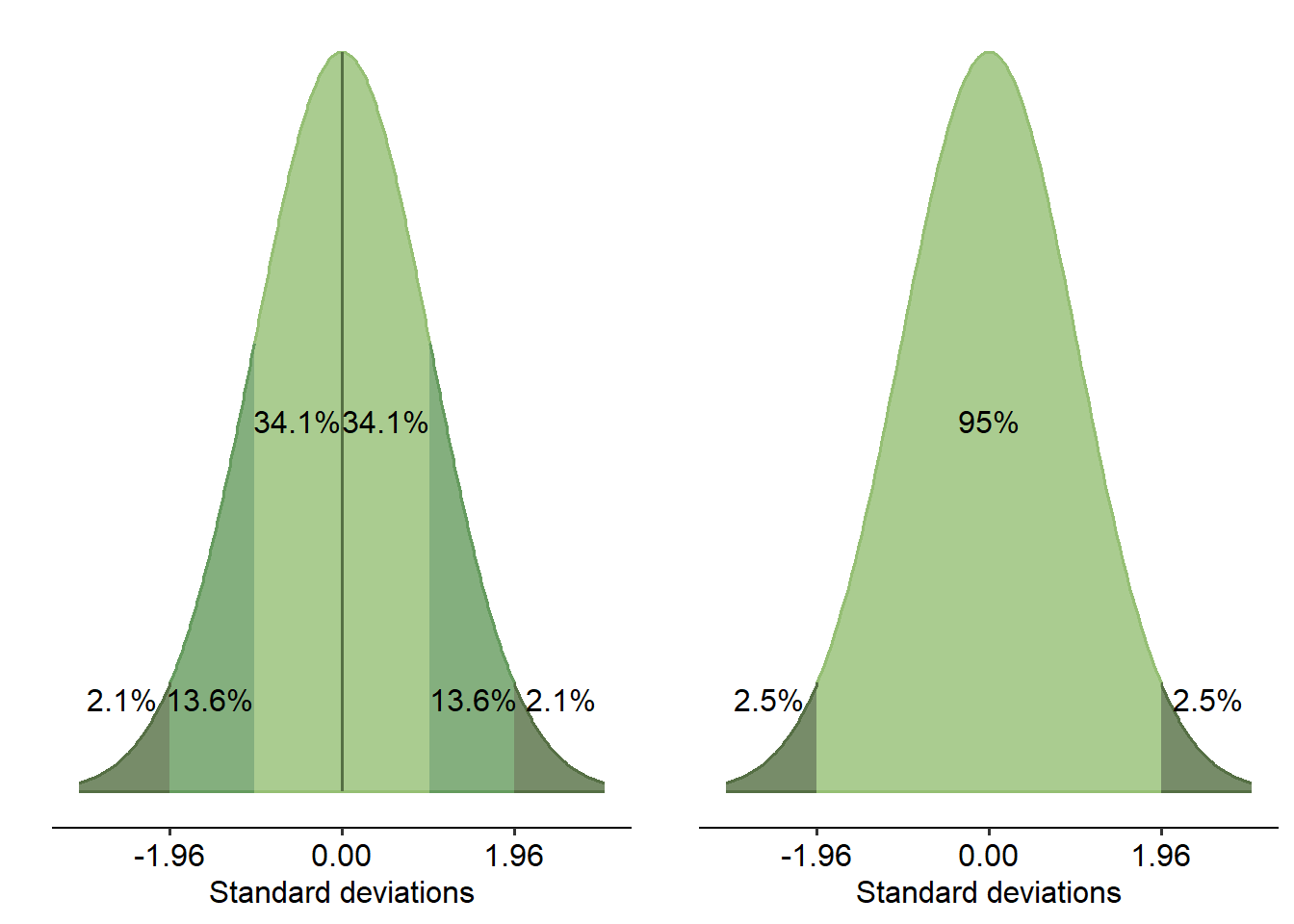
- We’ve talked a bit about the normal distribution and its properties - specifically, that 95% of your data lies within 1.96 SD either way of the mean
If you’ve got those concepts down, the rest of this page will be fairly straightforward.
3.6.1 z-scores
z-scores (z), sometimes called standard scores, are a measure that describe how many standard deviations a single data point is from the mean. If you recall the figure of the normal distribution from the previous page, notice how we quantify how much data is captured in terms of the number of standard deviations. z-scores are essentially this number - in other words, 95% of your data lies between z = -1.96 and z = 1.96.
The process of calculating z-scores is called standardisation. The primary utility of converting data into z-scores is that it becomes possible to compare data on different scales. Many statistical analyses employ some form of standardisation for a variety of reasons - some of which we’ll see in this subject.
3.6.2 Calculating z-scores
The formula for converting a raw data point into a z-score is:
\[ z = \frac{x - \mu}{\sigma} \]
Where x = an individual data point, \(\mu\) = mean and \(\sigma\) = SD.
For example - in their paper on the Goldsmiths Musical Sophistication Index, Mullensiefen et al. (2014) show that their general sophistication measure has a mean of 81.58, with an SD of 20.62. If a participant scores 100, we can calculate a z-score to see how many standard deviations they are away from the mean:
\[ z = \frac{100 - 81.58}{20.62} \] \[ z = 0.8933 \] A participant with a general sophistication score of 100 would be roughly 0.89 standard deviations away from the mean.
To z-score a vector in R, we use the scale() function. The scale() function takes two arguments: center, which determines whether the data is centered (i.e. subtracts the mean from each value), and scale, which essentially scales the data so the SD is 1. By default, both of these arguments are true.
##            [,1]
## [1,]  0.3806935
## [2,] -1.3324272
## [3,]  1.5227740
## [4,] -0.7613870
## [5,] -0.1903467
## [6,]  0.3806935
## attr(,"scaled:center")
## [1] 3.333333
## attr(,"scaled:scale")
## [1] 1.75119
3.6.3 Comparing across scales
As mentioned above, we can use z-scores to compare across measures on different scales. This becomes really useful when we want to compare two participants, for instance, or two different measures. This is simply done by calculating a z-score for each formula - as long as you know the mean and standard deviation of each scale as well.
As a simplistic example, let’s say we have two scales:
- Measure A sits on a scale of 0 - 100, with a mean of 50 and a standard deviation of 5
- Measure B sits on a scale of 0 - 80, with a mean of 45 and a standard deviation of 4
If a participant scores 40 on both scales, clearly we can’t compare them directly - a 40/100 is vastly different to a 40/80! But we could convert these into z-scores to see where the participant sits on each scale:
\(z_a = \frac{40 - 50}{5}\), and \(z_b = \frac{40 - 50}{5}\)
\(z_a = \frac{-10}{5}\), and \(z_b = \frac{-5}{4}\)
\(z_a = -2, z_b = -1.25\)
In other words, the participant’s z-score on Measure A is -2, and -1.25 on Measure B. Based on this, we can say that the participant scored slightly higher (relatively) on Measure B compared to Measure A.
A z-score lets us see how many standard deviations away from the mean a participant is. However, a more intuitive way of thinking about this is what percentile they sit in. To do this, we use something called a z-table. This z-table, in short, allows us to work out this percentage.
Most versions of the z-tables will present two separate z-tables: one for negative z-values, and one for positive z-values (credit: https://zoebeesley.com/2018/11/13/z-table/)
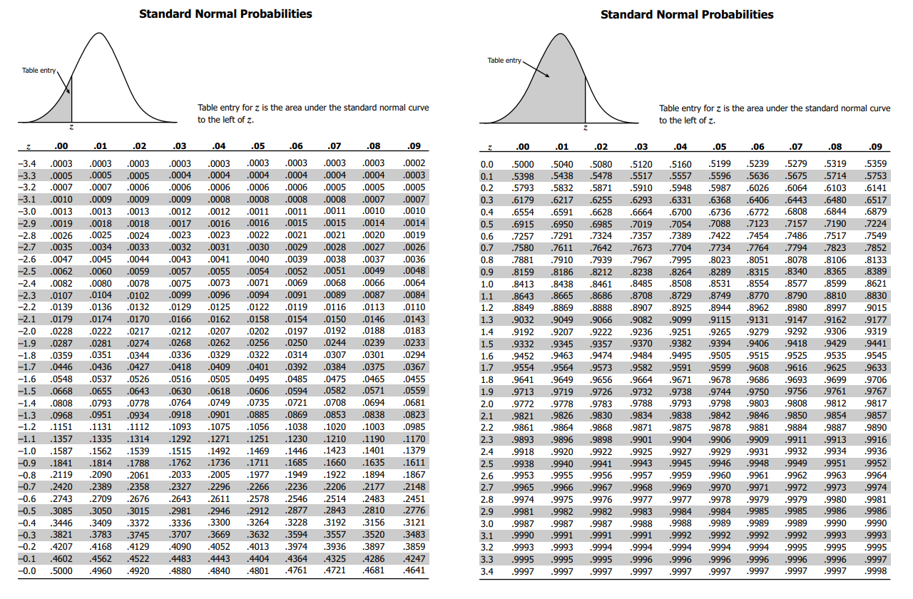
Here are the steps to read this table:
- Choose which table to read first. If you have a negative z-score, read the left one; if you have a positive z-score, read the right one.
- The rows and columns are basically arranged by decimal place. The rows index z-scores to 1dp, while the columns add the second decimal place. So, find the row first that corresponds to your z-score. In our example from above, our z-score was 0.89, so we want to find the row corresponding to 0.8.
- Next, find the column that corresponds to the second decimal place. We want to go all the way to the right-hand column labelled .09, to find the right column for our z-score of 0.89.
- Find the cell that corresponds to the row and column from above - that is the probability of getting a value below our z-score.
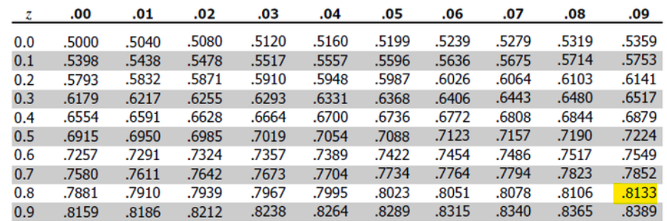
In this instance, our z-score of 0.89 has an associated probability of .8133, meaning that 81.3% of scores are below this z-score.
R, however, has a way of finding probabilities (percentiles) for z-scores for you. The pnorm() function calculates the probability of a specified value on a normal distribution. Given that z-scores follow the normal distribution, we can use pnorm() to calculate a given z-score’s associated probability.
The function is simple: it requires you to give the z-score (as argument q), the mean and standard deviation of the normal distribution you are interested in. By default, the mean is set to 0 and the SD set to 1, which is what we want for a z-score.
## [1] 0.8132671