8.3 Least squares regression
Linear regression starts with trying to fit a line to our continuous data. But… how on earth do we figure out where that line sits?
8.3.1 The regression line
See if you can take a guess where we should draw a line of best fit on the plot below:
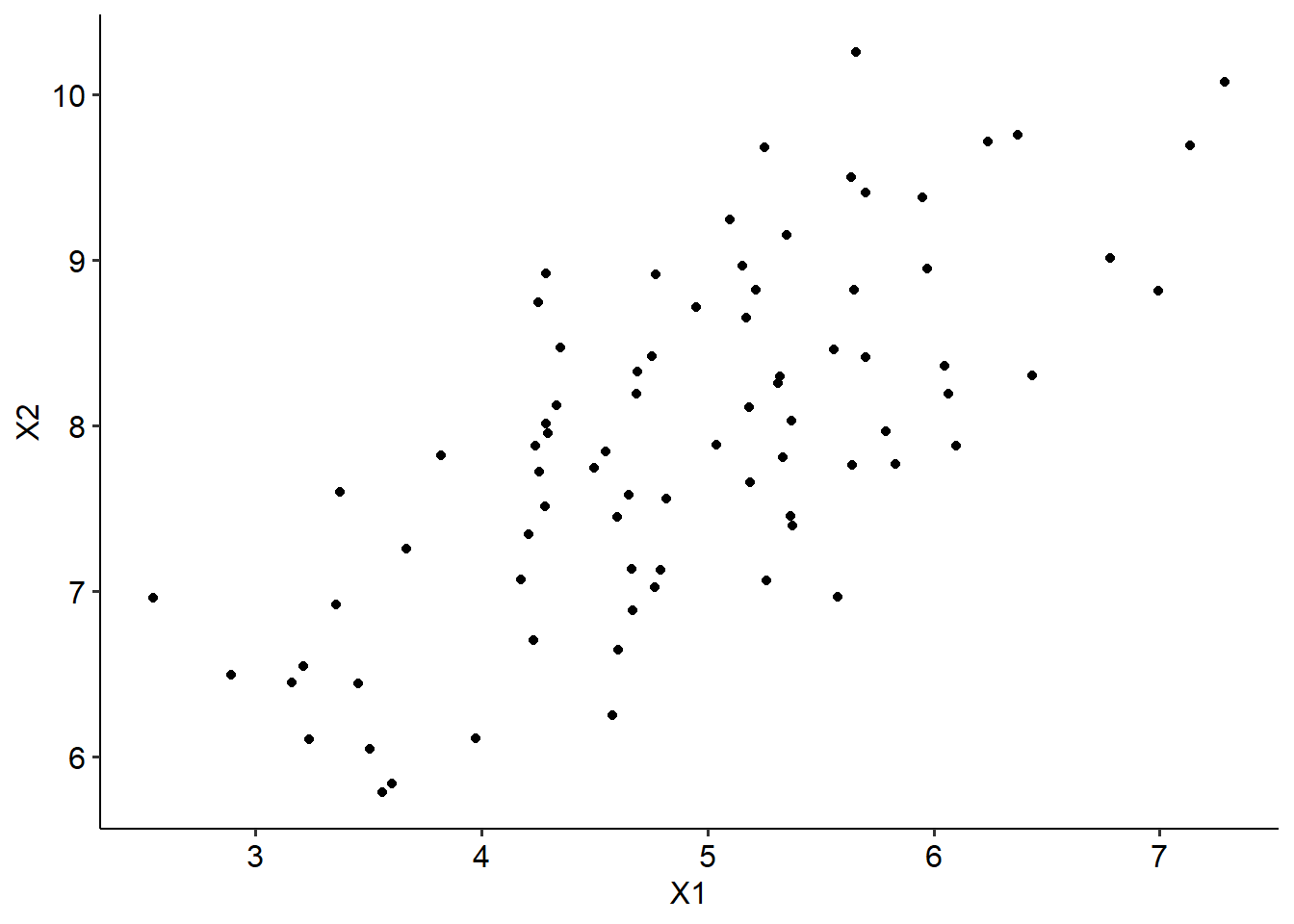
You might have some good guesses, and there’s every chance that you’ve drawn a line that fits the data points pretty well. But for this data, it’s pretty obvious where the line would sit, and the data that we do work with won’t always be as clear cut.
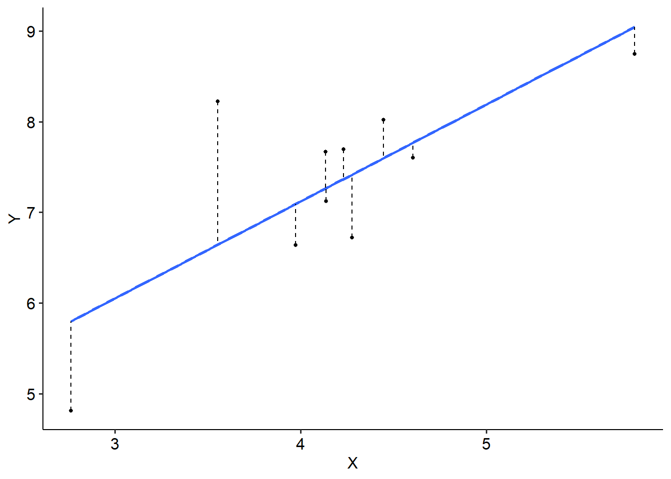
The line of best fit sits where the distance between the line and every point is minimised. See the example below, where we have 10 data points to illustrate. Each dot represents a single data point, while the solid blue line is our line of best fit. The dashed lines represent the difference between the blue line (which is what we predict - more on this later) and the actual data point. This difference is called a residual.
So, in other words, the line of best fit sits where the residuals are minimised.
We do this using the least squares principle. In essence, we calculate a squared deviation for each residual using the formula below - it might be familiar…
\[ SS_{res} = \Sigma (y_i - \bar y_i)^2 \]
Where \(y_i\) is each individual (ith) value on the y-axis, and \(\bar y_i\) is the predicted y-value (i.e. the regression line). Essentially, we calculate the residual for each data point, square it and add it all up.
The actual minimising part is something we won’t concern ourselves with for this subject (or at all), because quite frankly it’s complicated - the key here is to understand how a regression line is fit to the data.