6.4 Independent samples t-test
The independent-samples t-test is one of the most common tests that you will see in literature - it is one of the bread-and-butter tests of many music psychologists (for better or worse).
6.4.1 Independent samples
Independent samples t-tests are used when we want to compare two separate groups on one continuous outcome. They’re therefore well-suited for data with one categorical IV with two levels, against one continuous outcome.
6.4.2 Example data
For this example we’ll use a contrived but really simple example. A group of self-reported professional and amateur musicians were asked how many years of training they had on their primary instrument.
## Rows: 60 Columns: 3
## ── Column specification ───────────────────────────────────
## Delimiter: ","
## chr (1): Group
## dbl (2): Participant, Years_training
##
## ℹ Use `spec()` to retrieve the full column specification for this data.
## ℹ Specify the column types or set `show_col_types = FALSE` to quiet this message.Let us start with a nice plot:
w8_training %>%
  group_by(Group) %>%
  summarise(
    mean = mean(Years_training, na.rm = TRUE),
    sd = sd(Years_training, na.rm = TRUE),
    se = sd/n()
  ) %>%
  ggplot(
    aes(x = Group, y = mean)
  ) +
  geom_point(size = 3) +
  geom_errorbar(aes(
    ymin = mean - 1.96*se,
    ymax = mean + 1.96*se
  ), width = 0.2) +
  theme_pubr()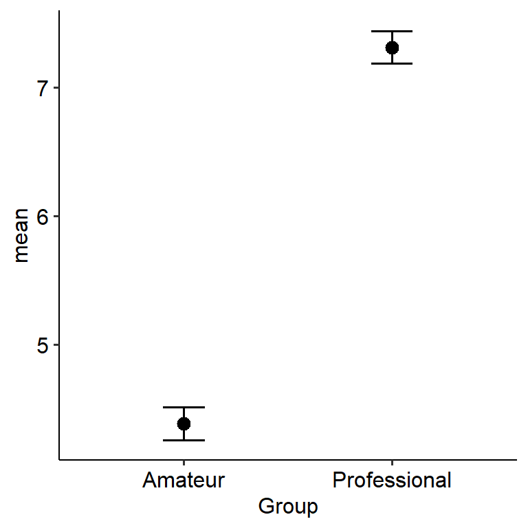
6.4.3 Assumption checks
There are three main assumptions for a basic independent samples t-test:
- Data must be independent of each other - in other words, one person’s response should not be influenced by another. This should come as a feature of good experimental design.
- The equality of variance (homoscedasticity) assumption. The classical t-test assumes that each group has the same variance (homoscedasticity). We can test this using a significant test called Levene’s test. If the test is significant (p < .05), the assumption is violated. In our data, this assumption seems to be intact (F(1, 58) = .114, p = .737).
## Warning in leveneTest.default(y = y, group = group, ...): group coerced to
## factor.- The residuals should be normally distributed. This essentially has implications for how well the data behaves. We can test this in two ways. The first is using a normality test, like the Shapiro-Wilks (SW) test, which is usually done using
shapiro.test(). Like Levene’s test, if the result of this test is significant it suggests that the normality assumption is violated. The result that Jamovi gives is not super clear in terms of what values exactly have been used to run the SW-test, so we will turn to another method.
For an independent t-test specifically, another way of testing this assumption is to simply see whether the dependent variable is normally distributed in both groups separately. In other words, we perform a Shapiro-Wilks test on years of training in both amateurs and professionals.
rstatix provides its own version of the SW-test (shapiro_test) that is compatible with group_by() and general tidyverse notation. Thus, we can first group using group_by(), and then run a SW-test on each group:
We can therefore see that for professionals our data is normally distribution (W = .94, p = .090), but not for amateurs (W = .90, p = .008).
6.4.4 Output
In reality, it’s rare that any of these assumptions are fully met even when tests say they are (the tests we just mentioned can be biased). This is especially true for classical t-tests, which are very sensitive to violations. A consistently better alternative is to use the Welch t-test, which assumes the equality of variance assumption is not met. Welch t-tests are also fairly robust against the normality assumption, and so are more flexible without sacrificing accuracy.
Here’s our output from R. Note that this is from a Welch t-test - R will do this by default.
##
##  Welch Two Sample t-test
##
## data:  Years_training by Group
## t = -5.8586, df = 57.989, p-value = 2.33e-07
## alternative hypothesis: true difference in means between group Amateur and group Professional is not equal to 0
## 95 percent confidence interval:
##  -3.922048 -1.924448
## sample estimates:
##      mean in group Amateur mean in group Professional
## 4.387097 7.310345Now for the effect size. For an independent samples t-test, you can give it almost the same as the regular t.test() function. The only change is that by default, cohens_d() will calculate Cohen’s d assuming equal variance. In order for our value of d to match a Welch-samples t-test, we need to set pooled_sd = FALSE (which makes the syntax slightly different to t.test()).
# Independent samples
# t.test(Years_training ~ Group, data = w8_training)
effectsize::cohens_d(Years_training ~ Group, data = w8_training, pooled_sd = FALSE)
Or again, we can alternatively use the cohen_d() function from rstatix:
From this, we can see that the two groups do significantly differ on years of training (t(57.99) = 5.86, p < .001). We can use the mean difference value to see, well… the difference in means between the two groups. In this case, professionals have 2.92 more years of training (on average; 95% CI = [1.92, 3.92]) compared to amateurs. So, we could write this up as something like:
An independent samples t-test was conducted to examine whether professionals and amateurs differed on years of musical instrument training. Professionals had on average 2.92 years more training (95% CI [1.92, 3.92]) compared to amateurs (t(57.99) = 5.86, p < .001), corresponding to a large significant effect (d = 1.51).
(n.b. the signs for t and the mean difference don’t overly matter so long as they are interpreted in the right way. The output above calculates amateurs - professionals, which is why the values for both are negative; but if you were to force the test to run the other way round, the values would be the same with the signs flipped. Hence why descriptives and graphs are super important too!)
If for some reason you do want R to run a Student’s t-test, you need to specify var.equal = TRUE. This tells R that we assume equality of variances.
##
##  Two Sample t-test
##
## data:  Years_training by Group
## t = -5.8424, df = 58, p-value = 2.476e-07
## alternative hypothesis: true difference in means between group Amateur and group Professional is not equal to 0
## 95 percent confidence interval:
##  -3.924805 -1.921691
## sample estimates:
##      mean in group Amateur mean in group Professional
##                   4.387097                   7.310345