5.3 Goodness of fit
Now that we’ve covered the conceptual groundwork for chi-square tests in general, we can now start looking at actual tests that can help us answer research questions. The most basic chi-square test is the goodness of fit test.
5.3.1 Goodness of fit tests
Goodness of fit tests are used when we want to compare a set of categorical data against a hypothetical distribution. Goodness of fit tests require one categorical variable - as the name implies, a goodness of fit test looks at whether the proportions of categories/levels in this variable fits an expected distribution. In other words, do our counts for each category match what we would expect under the null?
“Distribution” in this context means probability distributions, and can apply to a wide range of scenarios. For the purposes of what we’re learning here, we’ll stick to a question along the lines of: “do the categories of variable X align with their expected probabilities”?
5.3.2 Example
An example question that we look at in the seminar is Do Skittle bags have an even number of each colour? In the seminar, we go through whether or not a random bag has an even split of colours.
Here on Canvas, we’ll now tackle their equally delicious rivals, M&Ms. The data and analysis come courtesy of Rick Wicklin, a data analyst at SAS (who also make statistics software). You can read his full blog here: The distribution of colors for plain M&M candies. We’ll be recreating Rick’s first analysis here. We’re sticking with the candy theme because a) they’re delicious and b) the M&Ms are a great way to introduce what to do when expected proportions are not equal.
M&Ms come in six colours: red, blue, green, brown, orange and yellow. Unlike Skittles, these colours are not distributed equally within each bag of M&Ms. In 2008, Mars (the parent company) published the following percentage breakdown of colours:
- 13% red
- 20% orange
- 14% yellow
- 16% green
- 24% blue
- 13% brown
Rick collected his data in 2017, and so was interested in seeing if the proportions observed in his 2017 sample of M&Ms aligned with the distribution of colours listed in 2008.
A goodness of fit is the perfect test for this scenario because:
- We are making a claim about a distribution
- Our variable (colour) is categorical
- A chi-square goodness of fit will allow us to test whether the distribution of colours in a sample of M&Ms aligns with the published proportions.
Here’s our dataset:
5.3.3 Calculating \(\\\chi^2\)
In goodness of fit tests, we first calculated the expected frequencies. In this example though, the expected proportions aren’t equal - and so we have to be mindful of this when calculating expected values. See the expected count cell for Red M&Ms for how expected value is worked out in this instance.
We can draw this up in table form alongside our own data:
| Colour | Observed | Expected proportion | Expected count |
|---|---|---|---|
| Blue | 133 | 0.24 | 170.88 |
| Brown | 96 | 0.13 | 92.56 |
| Green | 139 | 0.16 | 113.92 |
| Orange | 133 | 0.20 | 142.4 |
| Red | 108 | 0.13 | \(712 \times 0.13 = 92.56\) |
| Yellow | 103 | 0.14 | 99.68 |
Then we would use the formula we saw on the previous page to calculate a chi-square statistic. However, since we’re doing this in R we’ll skip the manual maths.
\[ \chi^2 = \Sigma \frac{(O-E)^2}{E} \]
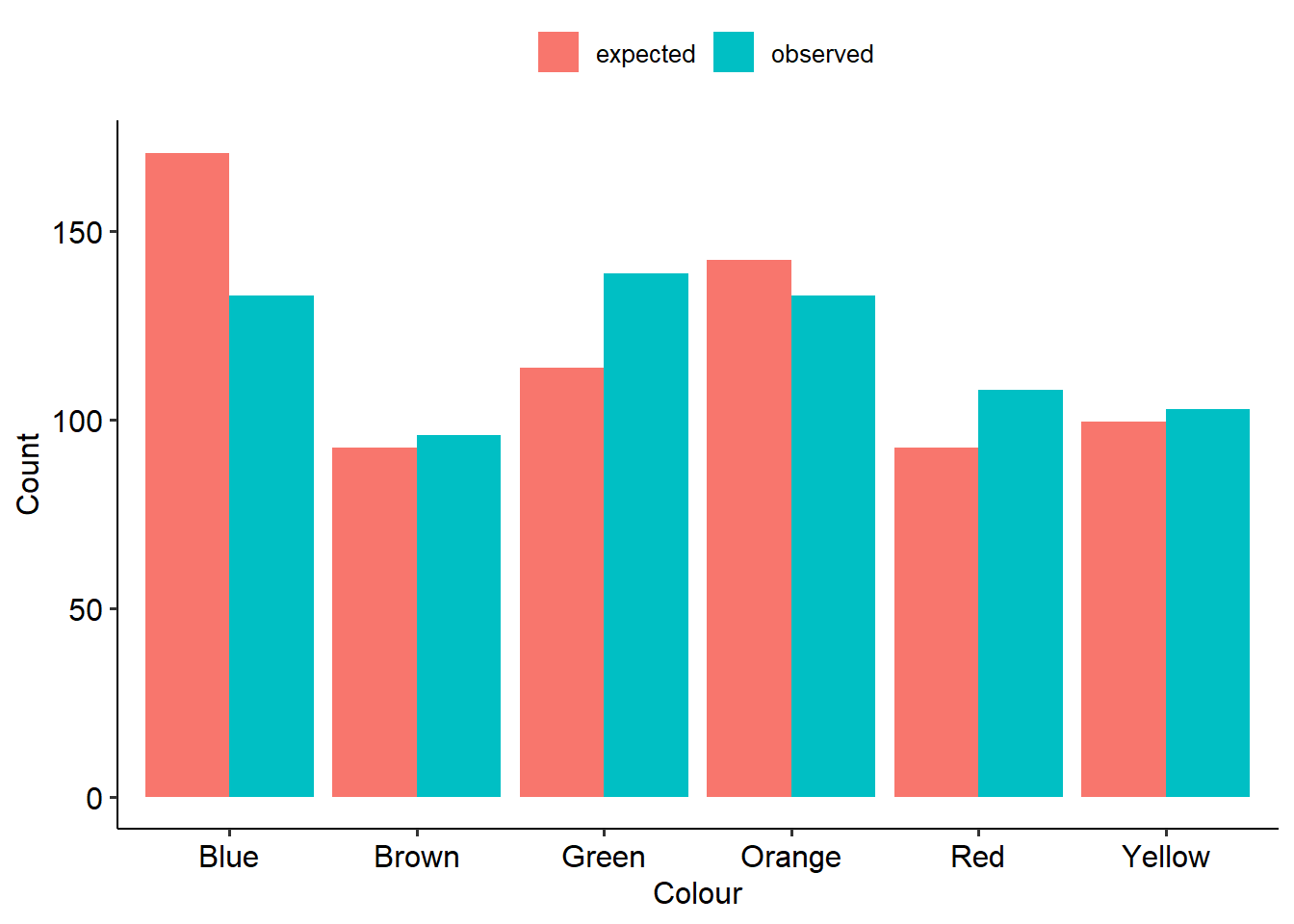
If we have a look at the observed vs expected values, we might have a good idea of what’s going on already:
5.3.4 Using R
The relevant function for doing a chi-square test in R is the chisq.test() function.4
By default, the chisq.test() function in R will assume that your categories have an equal chance of happening. However, in this instance we know that the colours are not evenly distributed. To ensure the proper probabilities are set beforehand, this needs to be specified by giving the p argument within chisq.test(). Note that the order of the expected probabilities needs to match the order they appear in the dataset (R will generally order these alphabetically unless told otherwise):5
5.3.5 Output
Here’s what our output looks like. First is our table of proportions. This can be really useful in laying out the data and seeing where the differences between observed and expected proportions might lie.
##
##   Blue  Brown  Green Orange    Red Yellow
## 133 96 139 133 108 103## Blue Brown Green Orange Red Yellow
## 170.88 92.56 113.92 142.40 92.56 99.68Next, here is our test output. The result is significant (p = .004), suggesting that the 2017 bag of M&Ms does not follow the same distribution of colours as the 2008 values. (If you read the rest of Rick’s blog post, it turns out that somewhere between 2008 and 2017 they changed where M&Ms are made, and actually split production across two factories that produce different distributions of colours. Rick eventually found out that his bag most likely came from one of the plants, although Mars has not made these proportions public like they used to.)
##
##  Chi-squared test for given probabilities
##
## data:  w7_mnm_table
## X-squared = 17.353, df = 5, p-value = 0.003877
Here is an example write-up of these results:
A chi-square test of goodness of fit was conducted to see whether the number of M&Ms aligned with the expected proportions published in 2008. There was a significant difference between the observed and expected proportions (\(chi^2\)(5, N = 712) = 17.35, p = .004). There were more green M&Ms and less blue M&Ms than expected.
There is an analogous function called
chisq_test()in therstatixpackage, but the base Rchisq.test()is easy enough to learn.↩︎If you need to order your variable a certain way, you should use the
factor()function. You will need to specify alevelsargument, which describes the ordering of the categories/groups, and optionally alabelsargument which gives each one a label. Both arguments take vectors, i.e.labels = c("1", "2", "3").↩︎