10.6 Semipartial correlations

10.6.1 Semipartial correlations (sr)

Semipartial correlations are similar in nature to partial correlations, with one key difference: the effect of the control variable Z is removed from X or Y, but not both. In other words, the controlling/partialling out of the effect of Z happens on only one of the two variables in the correlation.

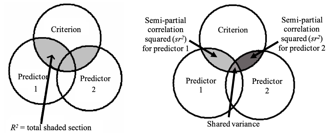
This property of semipartial correlations makes it particularly useful in multiple regressions. Imagine we have a multiple regression with outcome Y and two predictors X and Z. The amount of variance explained in Y - this is \(R^2\) - is a combination of the effects of individual predictors, and the relationship between predictors. Each predictor will contribute unique explained variance to that total amount of explained variance, and there will be some shared variance due to the relationship between predictors.

In other words, the \(R^2\) for a given multiple regression can be broken down into:

The unique variance explained by each predictor
The shared variance between predictors, due to the relationship between the predictors

If we wanted to find out how much X uniquely contributes to outcome Y, we could first calculate a semipartial correlation between X and Y, controlling for Z’s effect on X. In essence, by removing Z’s effect on X only, we are isolating any effect of X on Y specifically, allowing us to examine how much X is contributing on its own. Likewise, if we wanted to find out the unique variance explained by Z, we would run another semipartial between Z and Y, controlling for X’s effect on Z.

Squaring each sr value (i.e. calculate \(sr^2\)), will give the unique amount of variance explained by predictor X, after controlling for all other variables. If \(sr^2\) for variable X is 0.1, for instance, this means that 10% of the variance in Y is uniquely estimated/contributed by X. In turn, if we calculate \(sr^2\) values for each predictor, controlling for all other predictors, and subtract this from \(R^2\), this will give us the shared variance.

The diagram below summarises this info (shoutout to UQ:

10.6.2 Example

As an example, let’s look at a regression where Gold-MSI scores, openness to experience and trait anxiety predict flow proneness. In this model, \(R^2\) is .297, meaning that 29.7% of the variance is explained by all three predictors together.

The ppcor package provides a function called spcor.test(), which works just like its pcor.test() cousin. The only difference is that because we are now partialling the effect of control variables from the predictor only, the order in which we enter x and y matters.

Namely, x must be the outcome variable, and y must be the predictor we are interested in controlling. This ensures that the control variables are correctly being removed from the predictor variable and not the outcome:

spcor.test(
  x = flow_data$DFS_Total,
  y = flow_data$GoldMSI,
  z = flow_data[, c("openness", "trait_anxiety")]
)

Note that flow_data[, c("openness", "trait_anxiety")] is simply base R notation for selecting the columns named “openness” and “trait_anxiety” from the flow_data dataframe.

The semipartial correlation sr between Gold-MSI and flow proneness, controlling for the other two predictors (openness and trait anxiety) is sr = .401, p < .001.

To calculate \(sr2\) you will need to square the sr value above, which is thankfully easy enough in R:

0.4008732^2

## [1] 0.1606993

Squaring sr = .401 gives us \(sr^2\) = 0.1697; this means that Gold-MSI scores uniquely explain 17% of the variance in flow proneness.

10.6.3 Calculating all \(sr^2\) values

We could continue to use the spcor.test() function to calculate the other semipartial correlations for the other predictor and the outcome. However, just like pcor() we have an analogous function called spcor() that will calculate multiple semipartials in one go, using all of the variables in a provided dataframe. Like pcor(), the semipartials between two variables will be controlled for all other variables in the dataframe. In the output below, for example, the semipartial between DFS_Total and GoldMSI controls for both openness and trait_anxiety:

flow_data %>%
  dplyr::select(GoldMSI, trait_anxiety, openness, DFS_Total) %>%
  spcor()

## $estimate
##                 GoldMSI trait_anxiety    openness  DFS_Total
## GoldMSI       1.0000000    0.09414456  0.19909165  0.4120839
## trait_anxiety 0.1025177    1.00000000 -0.10654766 -0.3051688
## openness      0.2178267   -0.10705287  1.00000000  0.0725823
## DFS_Total     0.4008732   -0.27262017  0.06453483  1.0000000
## 
## $p.value
##                    GoldMSI trait_anxiety     openness    DFS_Total
## GoldMSI       0.000000e+00  7.371908e-03 1.121410e-08 1.652919e-34
## trait_anxiety 3.510562e-03  0.000000e+00 2.409483e-03 6.738338e-19
## openness      3.815754e-10  2.296393e-03 0.000000e+00 3.901925e-02
## DFS_Total     1.391025e-32  2.971642e-15 6.655997e-02 0.000000e+00
## 
## $statistic
##                 GoldMSI trait_anxiety  openness DFS_Total
## GoldMSI        0.000000      2.686366  5.771281 12.847970
## trait_anxiety  2.927722      0.000000 -3.044107 -9.103407
## openness       6.340209     -3.058708  0.000000  2.067352
## DFS_Total     12.430399     -8.049422  1.837118  0.000000
## 
## $n
## [1] 811
## 
## $gp
## [1] 2
## 
## $method
## [1] "pearson"

Recall that for a semipartial, we are interested in controlling the effect of other variables on the predictor and not the outcome. To obtain the corresponding values, we read across the row labelled with the outcome - i.e. DFS_Total - because this shows the semipartial correlation with each predictor in the columns.

We can see that the semipartial correlation between flow proneness and openness is not significant (sr = .07, p = .067), but the semipartial correlation with trait anxiety is (sr = -.27, p < .001). Squaring these values respectively gives us the following values:

\(sr^2\) for openness: 0.004 (i.e. 0.4% of variance in flow proneness)
\(sr^2\) for trait anxiety: 0.075 (i.e. 7.5% of variance in flow proneness)

If we now add all of our \(sr^2\) values together, we get 0.161 + 0.004 + 0.075 = 0.249, which means that 24% of the variance in flow proneness is due to the unique effects of the individual predictors. Subtracting this number from the value for \(R^2\) gives us 0.296 - 0.24 = 0.056, meaning that 5.6% of the variance in flow proneness is explained by the shared variance of all three predictors.

Sometimes, it is useful to present \(sr^2\) values for each predictor as part of a standard multiple regression table. This allows a reader to see how much each predictor is contributing to the variance in the outcome. in our case, we can say that Gold MSI scores explain the most variance in the outcome, while openness accounts for very little on its own.