11.3 Example
Below is a dataset relating to the presence of sleep disorders (credit to Laksika Tharmalingam on Kaggle for this dataset!), and various metrics relating to lifestyle and physical health. The dataset contains the following variables:
- id: Participant id
- gender: Participant gender
- age: Participant age
- sleep_duration: The number of hours the participant sleeps per day
- sleep_quality: The participant’s subjective rating (1-10) of the quality of their sleep
- physical_activity: How many minutes per day the participant does physical activity
- stress: Subjective rating of stress level (1-10)
- bmi: BMI category (Underweight, normal, overweight)
- blood_pressure: systolic/diastolic blood pressure
- heart_rate: Resting heart rate of the participant, in bpm
- sleep_disorder: Whether the participant has a sleep disorder or not (0 = No, 1 = Yes)
## Rows: 374 Columns: 11
## ── Column specification ───────────────────────────────────
## Delimiter: ","
## chr (3): gender, bmi, blood_pressure
## dbl (8): id, age, sleep_duration, sleep_quality, physical_activity, stress, ...
##
## ℹ Use `spec()` to retrieve the full column specification for this data.
## ℹ Specify the column types or set `show_col_types = FALSE` to quiet this message.
In this example, we’re interested in seeing whether specific factors predict whether or not the participant has a sleep disorder. We’ll work with an example with one predictor to start, and then move to multiple predictors afterwards.
11.3.1 Assumptions
The refreshing thing about the logistic regression is that there are actually very few assumptions that need to be made. For starters, we do not assume the following:
- Linearity between the IV and the DV
- Normality
- Homoscedasticity
None of these assumptions apply! What we do assume instead is:
- Linearity between the IV and the logit (i.e. the log odds)
- The outcome is a binary variable that is mutually exclusive (someone cannot be Y = 0 and Y = 1 at the same time)
- Absence of multicollinearity (in a multiple regression context)
11.3.2 Building the model
Here is where things start to change a little from what we’re used to. Because we are not building a linear model but a generalised linear model, we now need to use the glm() function in R. glm(), by and large, works exactly the same way as you have seen with lm(); you need to give it arguments in the form of outcome ~ predictor, and once you have run the function you need to call the results using summary(). The first thing that changes is that by virtue of the fact that we are using the GLM, we must specify what link function we are working with. This can be set using the family argument.
In the instance of logistic regression, the relevant family is binomial, and specifically binomial(link = "logit"):
The formula is a little strange, but binomial() is essentially a function that takes the argument link, for which we set the value as "logit". The logit argument is the default for this function though, so we can simply shorten this down to family = binomial specifically for logistic regressions. (For other binomial-based GLMs, you must specify the link.)
With that in mind, we can build our logistic regression models. In the first instance, let’s see if age predicts whether someone has a sleep disorder.
##
## Call:
## glm(formula = sleep_disorder ~ age, family = binomial, data = sleep)
##
## Coefficients:
##             Estimate Std. Error z value Pr(>|z|)
## (Intercept) -5.28024    0.65343  -8.081 6.44e-16 ***
## age          0.11549    0.01493   7.738 1.01e-14 ***
## ---
## Signif. codes:  0 '***' 0.001 '**' 0.01 '*' 0.05 '.' 0.1 ' ' 1
##
## (Dispersion parameter for binomial family taken to be 1)
##
##     Null deviance: 507.47  on 373  degrees of freedom
## Residual deviance: 433.36  on 372  degrees of freedom
## AIC: 437.36
##
## Number of Fisher Scoring iterations: 4
Note that our output table is a little bit different than what we’re used to; this is because of the change in procedure mentioned on the previous page (from least squares to maximum likelihood). However, we can still largely read this output the same way as we have. We can see that age is a significant predictor (p < .001).
The coefficient for age is .115. We can get the coefficients seperately by using the coef() function on our model:
## (Intercept)         age
##  -5.2802414   0.1154897
What does this mean? It means that for every 1 unit increase in age, the log odds increase by .115. This is important because remember that we’re modelling against log odds, not odds or probability! In essence, we have estimated the following:
\[ log(Odds) = -5.280 + (0.115 \times x_1) \]
We need to make sense of this another way somehow. Recall that log odds and odds relate to each other in the following way:
\[ Odds = e^{\beta_0 + \beta_1 x_1 + \epsilon_i} \]
To obtain the odds, as discussed on the previous page, we need to exponentiate our coefficients:
## (Intercept)         age
## 0.005091201 1.122423009
The exponentiated coefficient gives us our odds ratio. This describes the multiplied change in odds for every 1 unit increase of our predictor. In this instance, for every 1 year increase in age, the predicted odds of having a sleep disorder are multiplied by 1.12. Another way to describe this is that the predicted odds of having a sleep disorder increase by a factor of 1.12.
This coefficient does not mean the following:
- The odds increase by 1.12 for every unit of x - remember, only the log odds are linearly related to the predictor. The odds are non-linearly related.
- The probability increases by 1.12 - same deal as above, the probability isn’t linearly related to the predictors.
We can get confidence intervals around our estimated coefficients using confint(), just like we have previously. We can do this either on the original coefficients, or the exponentiated ones. The confidence interval around the exponentiated coefficients gives us a 95% CI for our odds ratio.This is probably more useful in terms of interpretation than the log odds coefficients, so we have chosen them here.
## Waiting for profiling to be done...## 2.5 % 97.5 %
## (Intercept) -6.60646431 -4.0395789
## age 0.08712071 0.1457569## Waiting for profiling to be done...## 2.5 % 97.5 %
## (Intercept) 0.001351603 0.01760488
## age 1.091028365 1.15691494Thus, we can say that the OR of a sleep disorder is 1.12 (95% CI = [1.09, 1.16]).
11.3.3 Predictions
Now recall that we can convert from odds to probabilities in the following manner:
\[ P(Y = 1) = \frac{1}{1 + e^{-(\beta_0 + \beta_1 x_1 + \epsilon_i)}} \]
Using this, we can make predictions about the probability of our outcome for a given value of our predictor. For example, what is the probability that a 50 year old will have a sleep disorder? That would be given as the following:
\[ P(Y = 1) = \frac{1}{1 + e^{-(\beta_0 + \beta_1 x_1 + \epsilon_i)}} \]
\[ P(Y = 1) = \frac{1}{1 + e^{-(-5.280 + (0.115 \times 50)}} \]
\[ P(Y = 1) = \frac{1}{1 + e^{-0.47}} \]
We can use R to do the calculation for us:
## [1] 0.6153838Thus, a 50 year old person has a 61.5% chance of having a sleep disorder (note that this has been rounded).
We can actually plot the expected probabilities across a range of values for age by first asking R to predict the probabilities across a range of ages. This will draw the characteristic S-shaped curve of the logistic model. We use the predict() function to calculate the predicted probabilities of each value of our predictor. The type = response argument is used here to tell R to predict the probabilities (and not the log odds).
## `geom_smooth()` using formula = 'y ~ x'## Warning in eval(family$initialize): non-integer #successes in a binomial glm!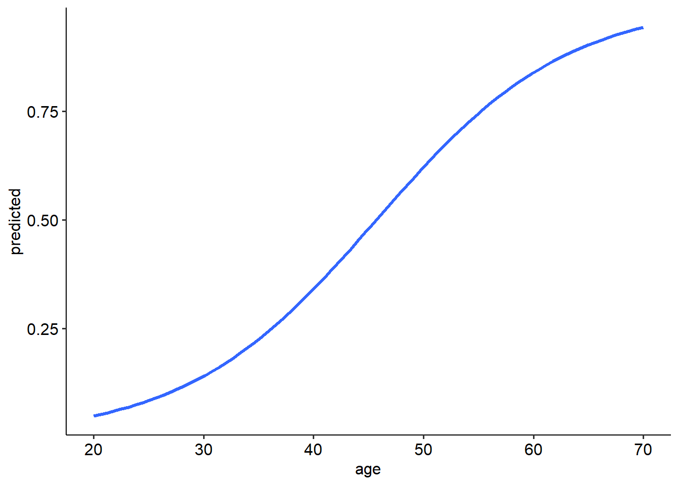
11.3.4 Logistic regression with multiple predictors
Let’s now expand out the previous example to include two predictors: age and stress. Just like a regular multiple regression, logistic regression can include multiple continuous predictors. This will take on the form of the following:
\[ log(Odds) = \beta_0 + \beta_1 x_1 + \beta_2 x_2 ... \beta_n x_n + \epsilon_i \]
This means that our odds formula becomes:
\[ Odds = e^{\beta_0 + \beta_1 x_1 + \beta_2 x_2 ... \beta_n x_n + \epsilon_i} \] And so on so forth with our probability formula. Really, this is just an extension of what we have already seen in multiple regression, but applied to a logistic regression context. Let’s see what this looks like in R with the below code:
sleep_glm2 <- glm(sleep_disorder ~ age + stress, data = sleep, family = binomial)
summary(sleep_glm2)
##
## Call:
## glm(formula = sleep_disorder ~ age + stress, family = binomial,
## data = sleep)
##
## Coefficients:
## Estimate Std. Error z value Pr(>|z|)
## (Intercept) -13.26171 1.41932 -9.344 < 2e-16 ***
## age 0.20510 0.02212 9.272 < 2e-16 ***
## stress 0.77585 0.10607 7.315 2.58e-13 ***
## ---
## Signif. codes: 0 '***' 0.001 '**' 0.01 '*' 0.05 '.' 0.1 ' ' 1
##
## (Dispersion parameter for binomial family taken to be 1)
##
## Null deviance: 507.47 on 373 degrees of freedom
## Residual deviance: 355.62 on 371 degrees of freedom
## AIC: 361.62
##
## Number of Fisher Scoring iterations: 5What do we see here? Well, we can see that age is a significant predictor of the presence of a sleep disorder (p < .001), and stress is as well (p < .001). Namely, for every year increase in age, the log odds of a sleep disorder increase by 0.205, holding stress constant. Likewise, for every 1 point increase in stress, the log odds increase by .776, holding age constant.
To convert this into odds ratios, we exponentiate the coefficients:
##  (Intercept)          age       stress
## 1.739856e-06 1.227649e+00 2.172449e+00
And let’s generate confidence intervals for our odds ratios too:
## Waiting for profiling to be done...## 2.5 % 97.5 %
## (Intercept) 9.083049e-08 0.0000240461
## age 1.178095e+00 1.2851325926
## stress 1.782252e+00 2.7038110976We can see that the for every 1 year increase in age, the predicted odds of having a sleep disorder increase by a factor (i.e. are multiplied by) of 1.23 (95% CI: [1.18, 1.29]), holding stress constant. For every 1 unit increase in stress, the predicted odds of a sleep disorder increase by a factor of 2.17 (95% CI: [1.78, 2.70]), holding age constant.
Just like before, we can also predict the probability that a participant will have a sleep disorder given their age and stress level. For example, let’s say we have a 50 year old with a stress level of 5:
\[ P(Y = 1) = \frac{1}{1 + e^{-(-13.262 + (0.205 \times 50) + (0.776 \times 5))}} \]
\[ P(Y = 1) = \frac{1}{1 + e^{-0.868}} = 0.704 \]
THus, this individual has a 70.4% chance of having a sleep disorder. Now what about if the person’s stress level is 6?
\[ P(Y = 1) = \frac{1}{1 + e^{-(-13.262 + (0.205 \times 50) + (0.776 \times 6))}} \]
\[ P(Y = 1) = \frac{1}{1 + e^{-1.644}} = 0.838 \] Now the person’s probability is 83.8%. In other words, it helps not to be stressed!