8.2 Regression hypotheses

Let’s move on from correlations to regressions, where we test whether one variable can predict another. To do that, let’s start by considering what a linear regression actually is, and how it works.

8.2.1 What is regression?

Recall the gestation versus birth weight example from the previous page:

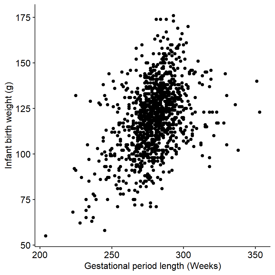
On the previous page, we saw that these two variables covary - as gestation length increases, the birth weight of the infant increases as well. We might then be interested in seeing whether gestational length predicts birth weight. In other words, does the gestational period of a pregnancy significantly predict the weight of the baby?

Regression is a technique that allows us to see whether one or more independent variables predict a (continuous) dependent variable. Regression is one of the most widely used techniques in psychology because we are often interested in relationships between continuous variables, and we are often interested in seeing whether certain variables predict others. Put simply, it allows us to examine relationships between variables (like correlations), but is a very flexible and powerful method of doing so.

Let’s kick off the regression portion of this module with a bit of terminology:

• The line is called the line of best fit. The slope of the line is, well, the slope. It describes how much Y changes if X changes by one unit.
• The point at which the line crosses the y-axis is called the intercept (the y-intercept in full). The intercept is one of the two paramaters of a regression line (the other being the slope).

In this module, we will also call the independent variable a predictor, and the dependent variable the outcome. The terms “predictor” and “outcome” are more general terminology than IV and DV, which are typically used in experimental contexts. However, they mean the same thing and can be used interchangeably.

8.2.2 How do regressions work?

Fundamentally, linear regressions involve plotting a line of best fit through the data. This line of best fit tells us something about the relationship between the two variables, including whether our predictor variable significant predicts the outcome.

See if you can take a guess where we should draw a line of best fit on the plot below:

You might have some good guesses, and there’s every chance that you’ve drawn a line that fits the data points pretty well. But for this data, it’s pretty obvious where the line would sit, and the data that we do work with won’t always be as clear cut.

The line of best fit sits where the distance between the line and every point is minimised. The difference between what we predict (the line) and an actual data point is called a residual, which simply refers to error. It makes sense then that to find the line of best fit, we want to place our line at the point where all of our possible residuals, or error, is minimised. If we didn’t minimise our error, we couldn’t say that it was the line of best fit!

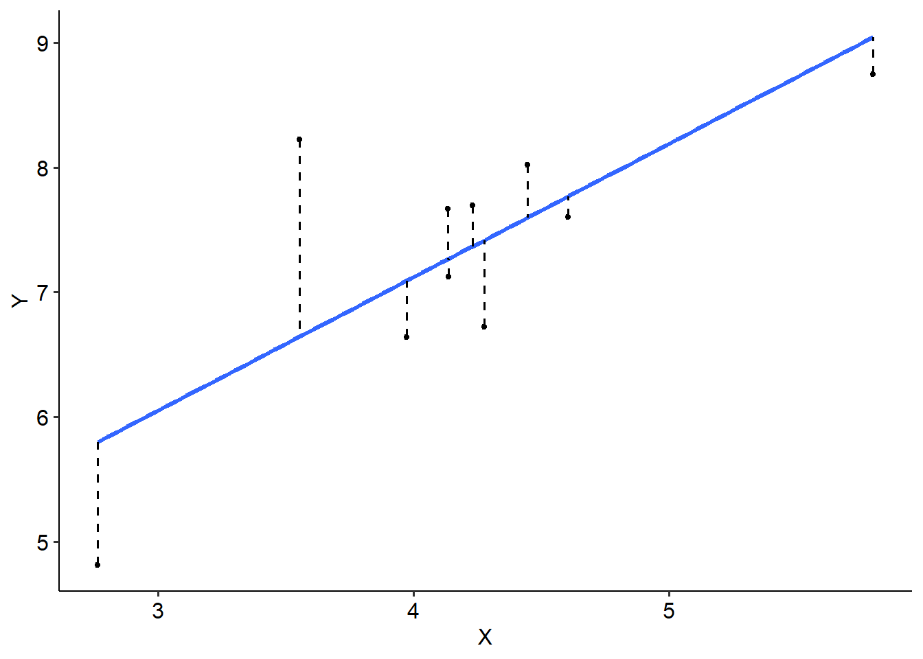
See the example below, where we have chosen 10 data points to illustrate. Each dot represents a single data point, while the solid blue line is our line of best fit. The dashed lines represent our residuals, or the difference between the blue line (what we predict) and each actual data point.

We do this using the least squares principle. In essence, we calculate a squared deviation for each residual using the formula below - it might be familiar…

\[ SS_{res} = \Sigma (y_i - \bar y_i)^2 \]

Where \(y_i\) is each individual (ith) value on the y-axis, and \(\bar y_i\) is the predicted y-value (i.e. the regression line). Essentially, we calculate the residual for each data point, square it and add it all up.

From there, we would fine the line where all of these squared deviations are minimised. The actual minimising part is something we won’t concern ourselves with for this subject, because it’s complicated - the key takeaway here is that the line of best fit sits at the point where we have minimised these residuals as much as possible.