12.6 Rotation, and interpreting output again
You may have noticed that on the previous page, we didn’t make much of an effort to actually talk about what the factors were or what they meant. That’s because the output that we got on the previous page isn’t actually terribly informative or easy to interpret. To help with this, in EFA we perform a technique called rotation.
12.6.1 Rotations
Rotations are a technique in EFA that are done to help with the interpretability of the factor solution. The key aim of rotation is to achieve simple structure where possible.
You may have noticed that the matrix from the previous page has quite a few variables with high enough loadings on multiple factors. This is called cross-loading, and indicates that two factors explain the variable. This is not easily interpretable! Ideally, in a robust simple structure we want:
- Only one loading per variable
- At least three loadings per factor
## Factor Analysis using method =  ml
## Call: fa(r = saq, nfactors = 3, rotate = "none", fm = "ml")
## Standardized loadings (pattern matrix) based upon correlation matrix
##        ML1    ML2    ML3    h2    u2  com
## q14  0.631               0.420 0.580 1.12
## q04  0.622               0.441 0.559 1.27
## q01  0.589  0.311        0.458 0.542 1.61
## q05  0.562               0.358 0.642 1.26
## q15  0.551               0.337 0.663 1.23
## q06  0.546         0.324 0.448 0.552 1.97
## q19 -0.371               0.229 0.771 2.27
## q22         0.314        0.238 0.762 2.88
## q02                0.319 0.229 0.771 2.84
##
##                         ML1   ML2   ML3
## SS loadings           2.333 0.474 0.352
## Proportion Var        0.259 0.053 0.039
## Cumulative Var        0.259 0.312 0.351
## Proportion Explained  0.738 0.150 0.111
## Cumulative Proportion 0.738 0.889 1.000
##
## Mean item complexity =  1.8
## Test of the hypothesis that 3 factors are sufficient.
##
## df null model =  36  with the objective function =  1.432 with Chi Square =  3674.737
## df of  the model are 12  and the objective function was  0.013
##
## The root mean square of the residuals (RMSR) is  0.012
## The df corrected root mean square of the residuals is  0.021
##
## The harmonic n.obs is  2571 with the empirical chi square  14.257  with prob <  0.285
## The total n.obs was  2571  with Likelihood Chi Square =  33.874  with prob <  0.000706
##
## Tucker Lewis Index of factoring reliability =  0.982
## RMSEA index =  0.0266  and the 90 % confidence intervals are  0.0163 0.0374
## BIC =  -60.351
## Fit based upon off diagonal values = 0.998
## Measures of factor score adequacy
##                                                     ML1    ML2    ML3
## Correlation of (regression) scores with factors   0.892  0.652  0.587
## Multiple R square of scores with factors          0.795  0.425  0.345
## Minimum correlation of possible factor scores     0.590 -0.150 -0.310
Rotation can help us achieve this. What rotations essentially do is change how variance is distributed within each factor. That wording is extremely important to note. It does not change our data in any way - the actual amount of variance explained by each factor does not change. What does change is how variance is distributed across the factors, which has the effect of then changing the loadings. But the actual data does not change!!
There are two families of rotations that we can employ.
- Orthogonal rotations force factors to be uncorrelated.
- Oblique rotations allow factors to be correlated.
The below diagram visualises what rotations do:
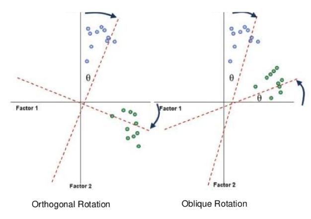
Which rotation to choose? In psychology, everything tends to be correlated with everything else, and it’s extremely rare that we would get an instance where two factors do not correlate at all. For that reason, oblique rotations are generally the way to go. Orthogonal rotations are extremely hard to justify without strong a-priori evidence - and even if two factors are uncorrelated, oblique rotations will give the same solution as orthogonal ones. In short, there’s generally no reason to prefer an orthogonal rotation by default.
12.6.2 Rotated factor solution
Let’s apply an oblique rotation to our factor analysis. The default oblique rotation is called oblimin. To do this, we need to re-run our fa() function with a rotation specified.
This produces the following output, which we now term a pattern matrix:
## Factor Analysis using method =  ml
## Call: fa(r = saq, nfactors = 3, rotate = "oblimin", fm = "ml")
## Standardized loadings (pattern matrix) based upon correlation matrix
##        ML1    ML3    ML2    h2    u2  com
## q01  0.714               0.458 0.542 1.02
## q04  0.609               0.441 0.559 1.06
## q05  0.553               0.358 0.642 1.02
## q06         0.704        0.448 0.552 1.01
## q14         0.440        0.420 0.580 1.57
## q15         0.434        0.337 0.663 1.32
## q02                0.506 0.229 0.771 1.04
## q22                0.488 0.238 0.762 1.08
## q19                0.412 0.229 0.771 1.11
##
##                         ML1   ML3   ML2
## SS loadings           1.360 1.043 0.756
## Proportion Var        0.151 0.116 0.084
## Cumulative Var        0.151 0.267 0.351
## Proportion Explained  0.431 0.330 0.239
## Cumulative Proportion 0.431 0.761 1.000
##
##  With factor correlations of
##        ML1    ML3    ML2
## ML1  1.000  0.591 -0.411
## ML3  0.591  1.000 -0.448
## ML2 -0.411 -0.448  1.000
##
## Mean item complexity =  1.1
## Test of the hypothesis that 3 factors are sufficient.
##
## df null model =  36  with the objective function =  1.432 with Chi Square =  3674.737
## df of  the model are 12  and the objective function was  0.013
##
## The root mean square of the residuals (RMSR) is  0.012
## The df corrected root mean square of the residuals is  0.021
##
## The harmonic n.obs is  2571 with the empirical chi square  14.257  with prob <  0.285
## The total n.obs was  2571  with Likelihood Chi Square =  33.874  with prob <  0.000706
##
## Tucker Lewis Index of factoring reliability =  0.982
## RMSEA index =  0.0266  and the 90 % confidence intervals are  0.0163 0.0374
## BIC =  -60.351
## Fit based upon off diagonal values = 0.998
## Measures of factor score adequacy
##                                                     ML1    ML3    ML2
## Correlation of (regression) scores with factors   0.718  0.672  0.636
## Multiple R square of scores with factors          0.515  0.452  0.405
## Minimum correlation of possible factor scores     0.031 -0.096 -0.190
Now we can see our simple structure taking effect, and this output is much more interpretable from before. These values are still regression coefficients between each latent factor and each variable, but now we can group these variables into their underlying latent factors much more easily. We can see that questions 1, 4 and 5 are best captured by factor 1, questions 6, 14 and 15 by factor 2 and questions 2, 19 and 22 by factor 3.
One warning here. On the previous page, where we had an unrotated solution, the communalities were calculated by summing the squared factor loadings for each variable. That rule no longer applies here because by allowing the factors to correlate, the regression loadings now capture non-specific variance. Summing the squared factor loadings will lead to greater communality values than what they actually are. However, as you can hopefully see in the uniqueness column, the actual communalities have not changed. Rotation does not change how much variance is explained in total - only how that variance is distributed!
Oblique rotations will also generate a factor correlation matrix. This calculates the correlations between the factors - remembering that by specifying an oblique rotation, we allowed them to correlate:
##            ML1        ML3        ML2
## ML1  1.0000000  0.5909483 -0.4107233
## ML3  0.5909483  1.0000000 -0.4475027
## ML2 -0.4107233 -0.4475027  1.0000000
Finally, we get the table of variance explained. This is now not as useful because of the same reason we cannot sum the squared factor loadings - each factor on its own now captures shared variance across the other factors as they are allowed to correlate. However, the total amount of variance explained is still 35.1%; once again, this does not change.
##                             ML1       ML3        ML2
## SS loadings           1.3601670 1.0425634 0.75593543
## Proportion Var        0.1511297 0.1158404 0.08399283
## Cumulative Var        0.1511297 0.2669700 0.35096287
## Proportion Explained  0.4306144 0.3300645 0.23932111
## Cumulative Proportion 0.4306144 0.7606789 1.00000000