3.4 Distributions
The ‘shape’ of our data is equally important. What does our data actually look like? Does it even matter what it looks like? The topic of distributions in statistics and probability can make up its own subject (in fact it does), but here we discuss the basics below.
3.4.1 The normal distribution
Earlier, we saw a series of graphs overlaid on top of each other. These graphs, while having different variability, were essentially all the same shape - they were symmetrical bell curves. These were all examples of the normal distribution (also called the Gaussian distribution). The classic normal distribution takes on a neat bell-shaped curve:
In the normal distribution, the majority of data points cluster in the middle, while all other values are symmetrically distributed from either side from the middle. This is what gives the normal distribution its recognisable bell shape.
The normal distribution is defined by two parameters: the mean and the standard deviation of the data. These two parameters define the overall shape of the bell curve - the mean defines where the peak is, while the standard deviation defines how spread out the tails are.
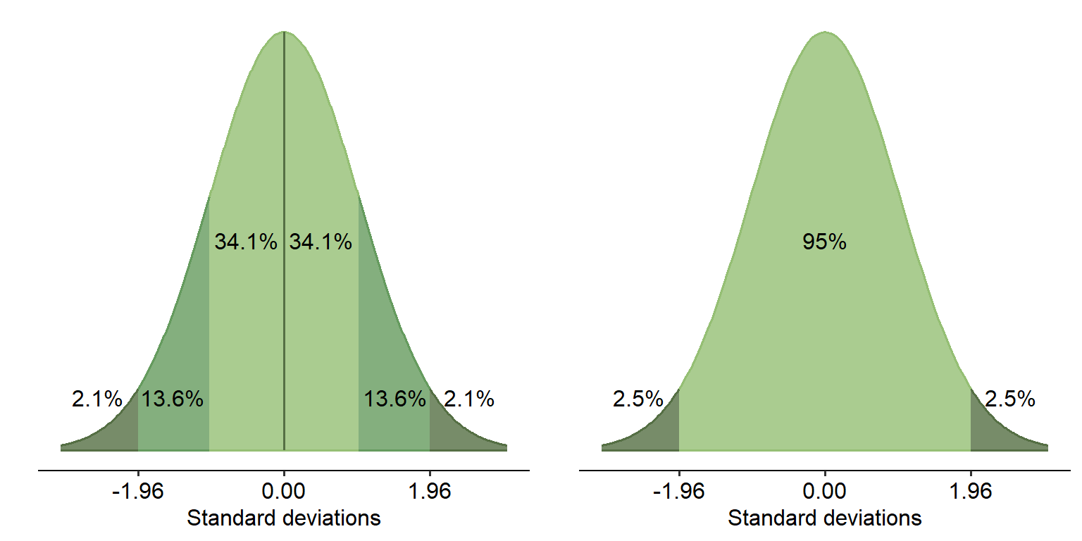
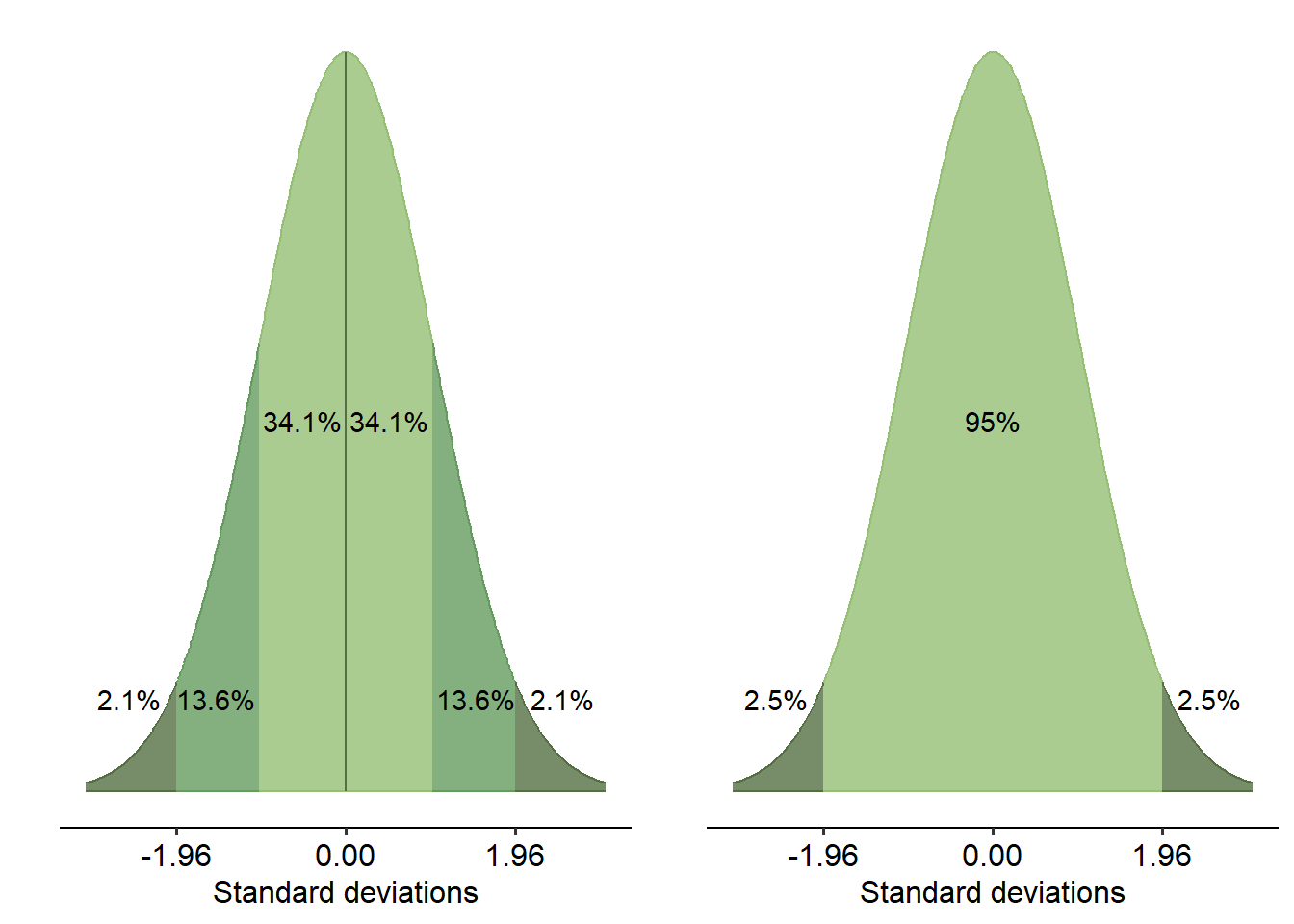
An important feature of the normal distribution is where all of the data is spread, regardless of its shape: 95% of the data within the curve falls within 1.96 standard deviations, either side of the mean. This applies to any normal distribution no matter what the scale of the data is. 99.7% of data falls within just below 3 standard deviations.
3.4.2 Graphing distributions
The slides below demonstrate a couple of ways in which you can graph distributions.
3.4.3 Skew
Skewness, as the name implies, describes whether or not a distribution is symmetrical or skewed. If a distribution is skewed, we would expect numbers to be bunched up at one end of the distribution. Have a look at the three graphs below:
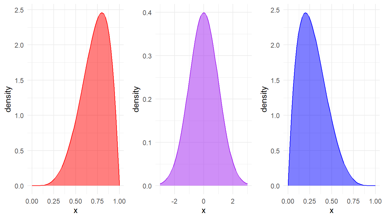
- The purple graph in the middle is symmetrically distributed, so we say that it has no skew.
- The red graph has values that are weighted towards the right-hand side of the x-axis, and so we say that it is either skewed left or negatively skewed.
- The blue graph, on the other hand is skewed right or positively skewed. The left-right refers to which end the tail of the distribution is on.
Skewness can also be quantified numerically:
- A skewness of 0 means that a distribution is normal
- A positive skew value means that the data is skewed right
- A negative skew value means that the data is skewed left
As a general rule, if a distribution has a skew greater than +1 or lower than -1, it is skewed. If your data is skewed then this is not the end of the world; it depends on the analysis you are performing, or what you are trying to do with the data. We will touch on this a bit more in coming weeks.
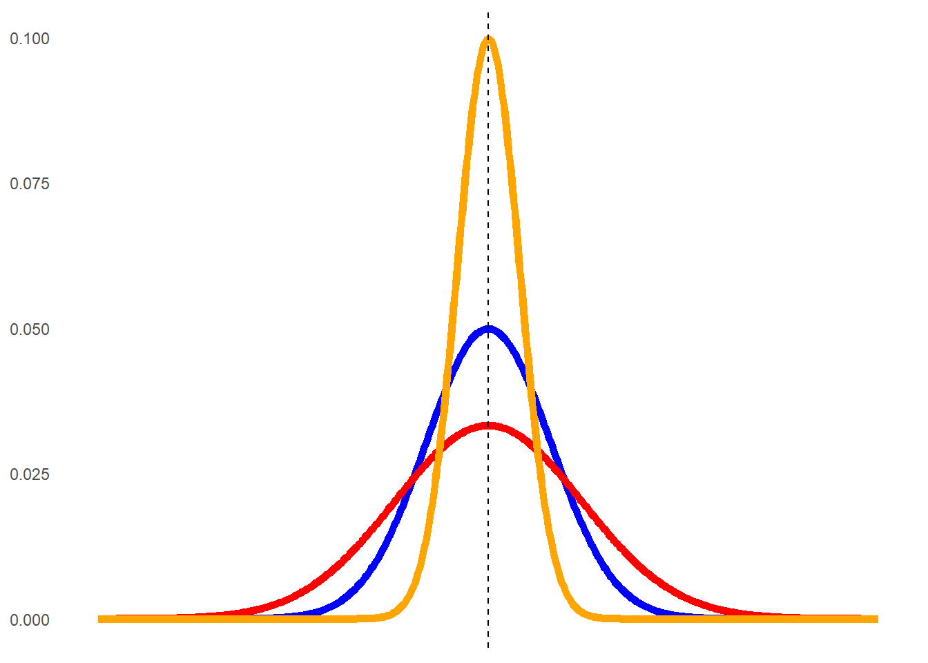
3.4.4 Kurtosis
Kurtosis refers to the shape of the tails specifically. Are all of the data bunched very tightly around one value, or are the data evenly spread out? The three graphs you saw up above all have different kurtoses.
The orange graph has most values very close to the peak at 50; therefore, the tails themselves are very small. The red line, on the other hand, is spread out and flatter so the tails are larger. The blue curve again approximates a normal distribution. We can quantify kurtosis through the idea of excess kurtosis - in other words, how far does it deviate from what we see in a normal distribution. This is shown below:
The different types of excess kurtoses are:
- Leptokurtic (heavy-tailed) - tails are smaller. Kurtosis > 1
- Mesokurtic - normally distributed. Kurtosis is close to 0
- Platykurtic (short-tailed) - tails are larger, and the peak is flatter. Kurtosis < -1
Therefore, in the example above the orange curve would be considered leptokurtic, while the red one would be platykurtic.
Below are a series of skewness and kurtosis values from three different data sets. For each:
- Determine if the data is skewed or not, and if so then what type of skew
- Determine the type of kurtosis
- Sketch a rough version of what this skew and kurtosis might look like (doesn’t have to be perfect!)
| Dataset A | Dataset B | Dataset C | |
|---|---|---|---|
| Skewness | 0.3209 | 5.2934 | -3.1945 |
| Kurtosis | -0.1023 | 10.9238 | -2.7263 |