6.3 One-sample t-test

The first test that we’ll look at is the one-sample t-test, which is the most simple of the three that we will look at this week.

6.3.1 One-sample t-test

A one-sample t-test is used when we want to compare a sample against a hypothesised population value. It is useful when we already know the expected value of the parameter we’re interested in, such as a population mean or a target value.

The basic hypotheses for a three-way interaction are:

• \(H_0\): The sample mean is not significantly different from the hypothesised mean. (i.e. \(M = \mu\))
• \(H_1\): The sample mean is significantly different from the hypothesised mean. (i.e. \(M \neq \mu\))

It’s worth noting that one-sample t-tests aren’t that commonly used because they require you to know the population value (or, if you hypothesise a value, you need to justify why). However, they’re included here because they’re still a part of the t-test family, and they serve as a nice introduction to how t-tests work.

6.3.2 Example data

Historically, scores in a fictional research methods class average at 72. This year, you are the subject coordinator for the first time, and you notice that last year’s cohort appear to have really struggled. You want to see if there is a meaningful difference between the cohort’s average grade and what the target grade should be.

Here’s the dataset below:

w8_grades <- read_csv(here("data", "week_8", "W8_grades.csv"))

## Rows: 128 Columns: 2
## ── Column specification ────────────────────────
## Delimiter: ","
## dbl (2): id, grade
## 
## ℹ Use `spec()` to retrieve the full column specification for this data.
## ℹ Specify the column types or set `show_col_types = FALSE` to quiet this message.

head(w8_grades)

6.3.3 Assumption checks

There is only one relevant assumption that we need to check for the one-sample t-test: whether our data is distributed normally or not. We can do this in two ways. The first and quickest is through a test called the Shapiro-Wilks test (often abbreviated as the SW test). The SW test is a significant test of departures from normality. The statistic in question, W, is an index of normality. If W is close to 1, then data is normally distributed; the smaller W becomes, the more non-normal the data is.

A significant p-value on the SW test suggests that the data is non-normal. Thankfully, that isn’t an issue here.

shapiro.test(w8_grades$grade)

## 
##  Shapiro-Wilk normality test
## 
## data:  w8_grades$grade
## W = 0.98652, p-value = 0.2395

The second way is through a Q-Q plot (Quantile-Quantile) plot. Essentially, these plot where data should be (if the data are normally distributed) against where the data actually is. If the normality assumption is intact, most of the data should lie on or close to the straight line, like the left plot. Data that looks like the right, where the data curves away from the central line, is more likely to be non-normally distributed.

To draw a Q-Q plot in R, the base functions qqnorm() and qqline() can be used. qqnorm() will draw the basic Q-Q plot, while qqline() will draw a straight line through the graph. Note that qqnorm() must be run first before qqline() can be used.

In this case, since we want to draw a Q-Q plot of a single variable, we just need to give the name of the column/variable we are interested in using data$variable format.

qqnorm(w8_grades$grade)
qqline(w8_grades$grade)

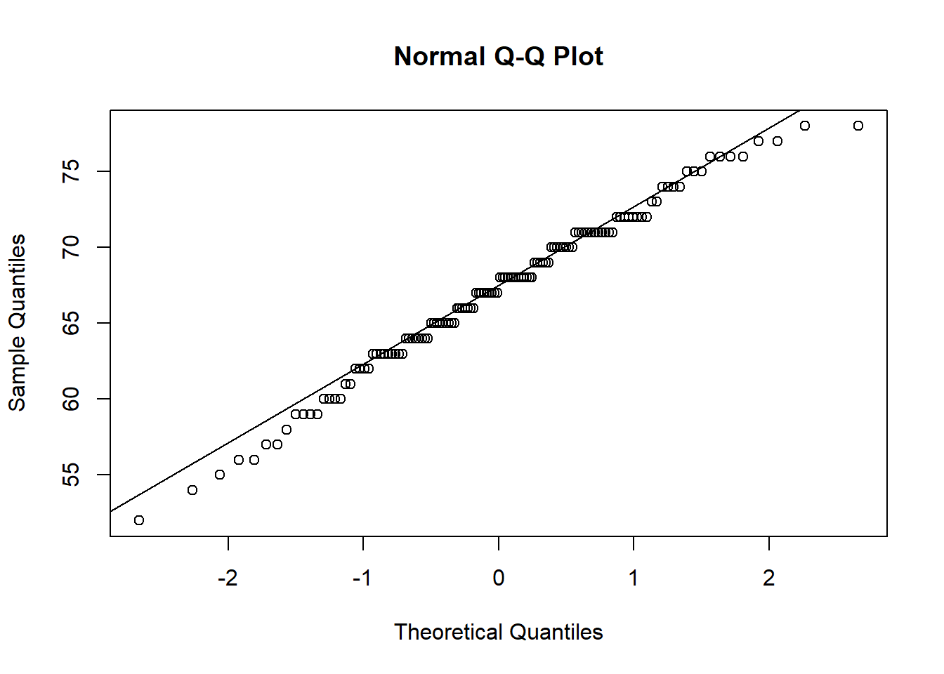
In our case, most of the points fall quite close to the main line, so we seem to be ok here - in line with our Shapiro-Wilks test (though this won’t always be the case).

6.3.4 Output

Here are our descriptive statistics. They alone might already tell us something is going on:

w8_grades %>%
  summarise(
    mean = mean(grade, na.rm = TRUE),
    sd = sd(grade, na.rm = TRUE),
    median = median(grade, na.rm = TRUE)
  ) %>%
  knitr::kable(digits = 2)

mean	sd	median
67.09	5.38	67.5

To run a one-sample t-test, the basic function is the t.test() function. For a one-sample t-test, you must provide the argument x (the data) and mu, which is the hypothesised population mean.

Below is our output from the one-sample t-test. Our result tells us that there is a significant difference between the mean of the sample (M = 67.09) and the hypothesised mean of 72 (p < .001). The mean difference here is calculated as Sample - Hypothesis; therefore, a difference of -4.91 means that the sample mean is 4.91 units lower than the population mean (which hopefully would have been evident from the descriptives anyway). This means that for some reason, last year’s cohort are performing worse than the expected average.

R Note: Jamovi will give you a 95% confidence interval around the mean difference as 95% CI = [-5.85, -3.97]. R however will give you a CI around the actual mean. In this case, the 95% confidence interval for the group mean is [66.15, 68.03]. Really though, this is giving us the same information; 72 - 5.85 = 66.15, and 72 - 3.97 = 68.03. So the only difference is in what value is presented for the 95% CI, but the actual inference itself doesn’t change.

t.test(w8_grades$grade, mu = 72)

## 
##  One Sample t-test
## 
## data:  w8_grades$grade
## t = -10.342, df = 127, p-value < 2.2e-16
## alternative hypothesis: true mean is not equal to 72
## 95 percent confidence interval:
##  66.14570 68.02617
## sample estimates:
## mean of x 
##  67.08594

Anoter way of writing a one-sample t-test is to use variable ~ 1 formula notation. The ~ 1 is used to indicate that we are running a one-sample t-test. We still need to define mu = 72 to set our hypothesised population mean.

t.test(grade ~ 1, data = w8_grades, mu = 72)

## 
##  One Sample t-test
## 
## data:  grade
## t = -10.342, df = 127, p-value < 2.2e-16
## alternative hypothesis: true mean is not equal to 72
## 95 percent confidence interval:
##  66.14570 68.02617
## sample estimates:
## mean of x 
##  67.08594

Alternatively, you can use the t_test() function in rstatix. This function also requires formula notation. detailed = TRUE will print a detailed output that will give the 95% CI for the mean as well:

w8_grades %>%
  t_test(grade ~ 1, mu = 72, detailed = TRUE)

As we have previously done for chi-square tests, we will want to calculate an effect size for our t-test. The cohens_d() function from effectsize can handle the calculation of effect sizes for all three variants of t-tests. One thing that’s quite nice about this function is that the required syntax for cohens_d() is nearly identical to that for t.test() - meaning that the correct type of Cohen’s d (one-sample, independent samples, paired) will be calculated based on what you put in.

For a one-sample t-test, for instance, you can write the syntax exactly as you would for t.test():

# One-sample
# t.test(w8_grades$grade, mu = 72)
effectsize::cohens_d(w8_grades$grade, mu = 72)

The alternate way of specifying a one-sample t-test, the var ~ 1 format, also works. cohens_d() will recognise both.

# One-sample - alternate
# t.test(grade ~ 1, data = w8_grades, mu = 72)
effectsize::cohens_d(grade ~ 1, data = w8_grades, mu = 72)

Alternatively, you can use the rstatix package. This will give the same values, but the confidence intervals generated by effectsize are traditional confidence intervals, whereas rstaix uses a different method (which we need not concern ourselves with). In any case, the actual width of the intervals should be similar. Just note that for paired samples Cohen’s d, long data is required (as is the case with t-tests in rstatix).

For a one-sample t-test, the formula once again needs to be in var ~ 1 format and mu must be specified:

w8_grades %>% 
  rstatix::cohens_d(grade ~ 1, mu = 72, ci = TRUE, ci.type = "norm") 

Here is an example write-up of the above:

A one-sample t-test was conducted to examine whether grades in the research methods class differed from the historical average of 72. The sample’s grades (M = 67.09, SD = 5.38) were significantly lower than the historical average (t(127) = -10.3, p < .001), with a mean difference of 4.91 (95% CI = [-5.85, -3.97]). This effect was large in size (d = -0.91).