14.2 Spearman’s rho

14.2.1 Introduction

Spearman’s rho (\(\rho\)) is a non-parametric correlation coefficient, broadly equivalent in interpretation with Pearson’s correlation coefficient. It is used to calculate a correlation in instances where Pearson’s r would not be appropriate; namely, when data is not linear.

Spearman’s rho can be used when data is monotonic. Monotonic data is data where as X changes, Y changes in one direction. Below is a visualisation of monotonic versus non-monotonic data:

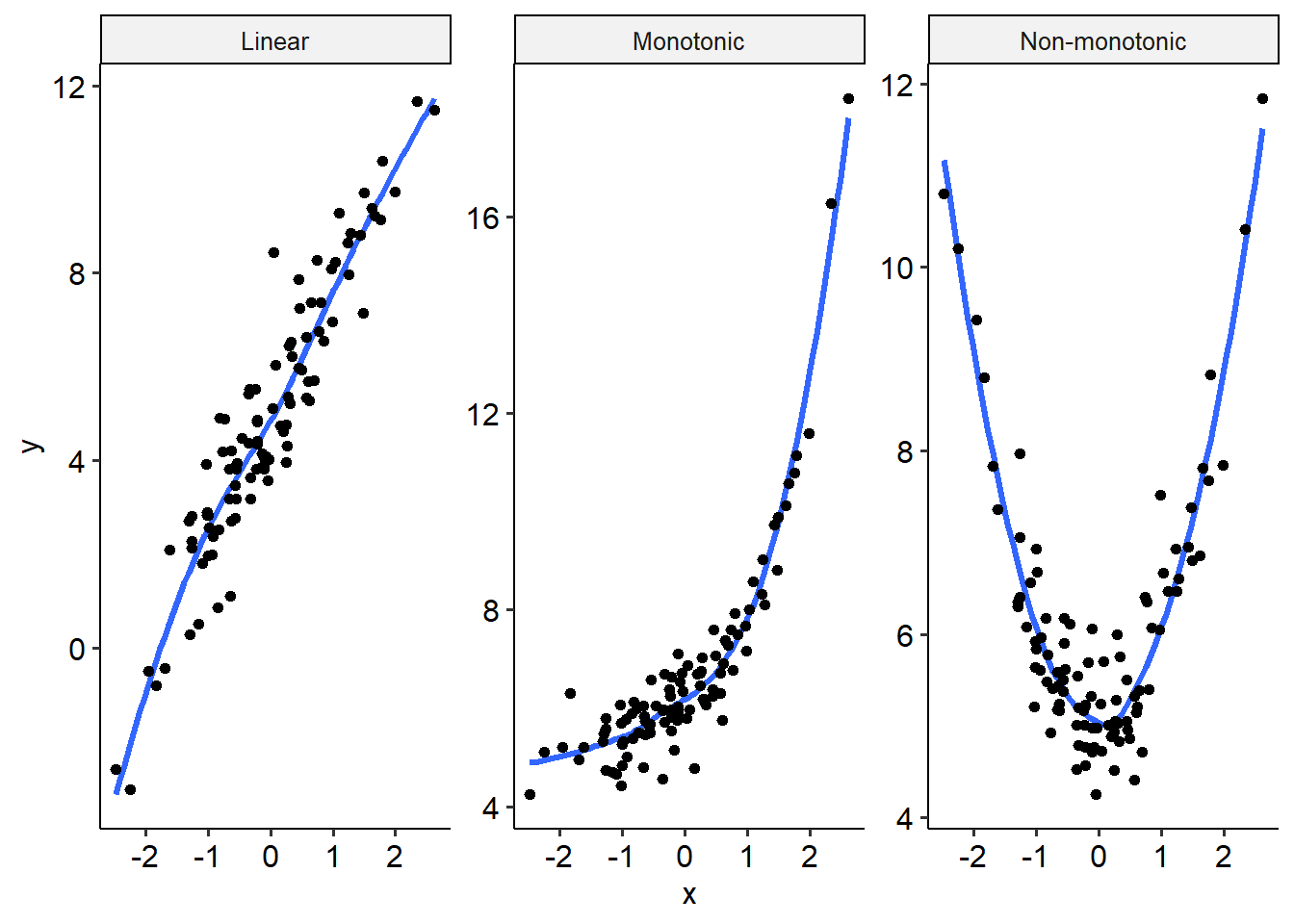
In the linear and monotonic examples, the line of best fit follows one direction - up. In the rightmost graph, however, there is a decrease and then an increase in the predicted values of y. This is an example of a non-monotonic function.

14.2.2 Understanding ranks

Non-parametric statistics, including all of the ones that we talk about in this module, rely on establishing ranks in your data. Mathematically, this is how non-parametric tests are able to test the hypotheses they do without needing to rely on accurately estimating some parameter, or making assumptions about said parameters. Although each test has a different way of using these ranks, many of them often start by calculating ranks in your data.

This is about as simple as it sounds. Consider the table below, with 5 measurements on a simple scale. The left column shows the raw data, while the middle column shows the ranked data - largest to smallest, reading top to bottom. The right column shows their ranks in order. The smallest value is given a rank of 1.

The ranks are then used to calculate test statistics for non-parametric tests.

14.2.3 Example

Below is a simple example of a correlation between two variables where non-linearity may be important. Singing accuracy is naturally skewed heavily, and develops non-linearly throughout life.

singing <- read_csv(here("data", "nonpara", "singing_data.csv"))

## Rows: 284 Columns: 2
## ── Column specification ────────────────────────
## Delimiter: ","
## dbl (2): accuracy, age
## 
## ℹ Use `spec()` to retrieve the full column specification for this data.
## ℹ Specify the column types or set `show_col_types = FALSE` to quiet this message.

The relevant dataset contains just two variables: accuracy (measured in cents) and age (participant age). The scatterplot below shows the relationship between these two variables:

singing %>%
  ggplot(
    aes(x = age, y = accuracy)
  ) +
  ggpubr::theme_pubr() +
  geom_point()

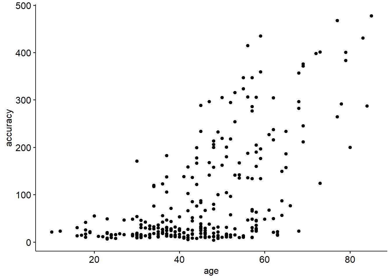
To calculate Spearman’s rho, the steps are much the same as the way they are for normal correlations - we use the same cor.test() function that we saw earlier. The main difference is that we now must specify the method argument to equal to "spearman", which will calculate Spearman’s rho instead.. Here, we see results consistent with a Pearson’s correlation; a significant, positive association between age and accuracy (\(\rho\) = .53, p < .001).

cor.test(singing$accuracy, singing$age, method = "spearman")

## Warning in cor.test.default(singing$accuracy, singing$age, method =
## "spearman"): Cannot compute exact p-value with ties

## 
##  Spearman's rank correlation rho
## 
## data:  singing$accuracy and singing$age
## S = 1808559, p-value < 2.2e-16
## alternative hypothesis: true rho is not equal to 0
## sample estimates:
##       rho 
## 0.5262664