12.4 How many factors/components?
A crucial element of doing an EFA is deciding on the number of factors that should be extracted for the final solution. This is not a trivial decision, and essentially determines the final factor structure you derive and interpret in your factor analysis. Note that while we mainly talk about factors on this page, the same considerations apply when thinking of components in PCA.
12.4.1 Deciding on the number of factors
Recall that an EFA/PCA will extract up to k factors/components, where k is the number of observed variables. At k factors/components, this will have explained all of the possible variance there is to explain in the observed variables. The basic idea behind how these factors are calculated is by essentially drawing straight lines through our data, much like a regression line. The idea is that each straight line (factor/component) should explain as much variance as possible, and each successive factor/component that is drawn explains the remaining variance.
The first factor/component will always attempt to explain the most variance possible. The second factor/component will then be drawn through what remains after the first factor/component is calculated, in a way that both maximises the variance captured and is uncorrelated with the first factor/component. This lets us capture as much variance as possible in a clean way, where we can identify the relative contributions of each successive factor/component.
The amount of variance that is captured by each factor/component is represented by a number called the eigenvalue. Naturally, the first factor/component will have the highest eigenvalue, and the eigenvalue of each factor/component afterwards will decrease.
This means that at some point, we reach a stage where an additional factor doesn’t add much in terms of the variance explained. This indicates that there isn’t much utility in retaining factors after a certain point - i.e. we get diminishing returns on increasing the number of factors we have to interpret. We must strike a balance between having a relatively straightforward factor structure to interpret and how much variance is explained. Too few factors means we may not accurately capture enough variance to be meaningful or miss very crucial relationships, but too many factors means we lose parsimony and interpretability.
There are several ways in which we can identify where the most optimal number of factors to retain is.
12.4.2 The Kaiser-Guttman rule
The Kaiser-Guttman, Kaiser or simply the “eigenvalue > 1” rule states that we should simply keep any factor with an eigenvalue above 1. To do this, we first need a correlation matrix from our data. We then feed this to the eigen() function in base R, which will calculate eigenvalues. I’ve piped it here, but you can also go straight to eigen(cor(saq)). Our data suggests that we retain 2 factors using this rule.
## [1] 2.9515869 1.2029159 0.9339932 0.7897083 0.7671243 0.6453702 0.6078335
## [8] 0.5663971 0.5350707
12.4.3 The scree plot
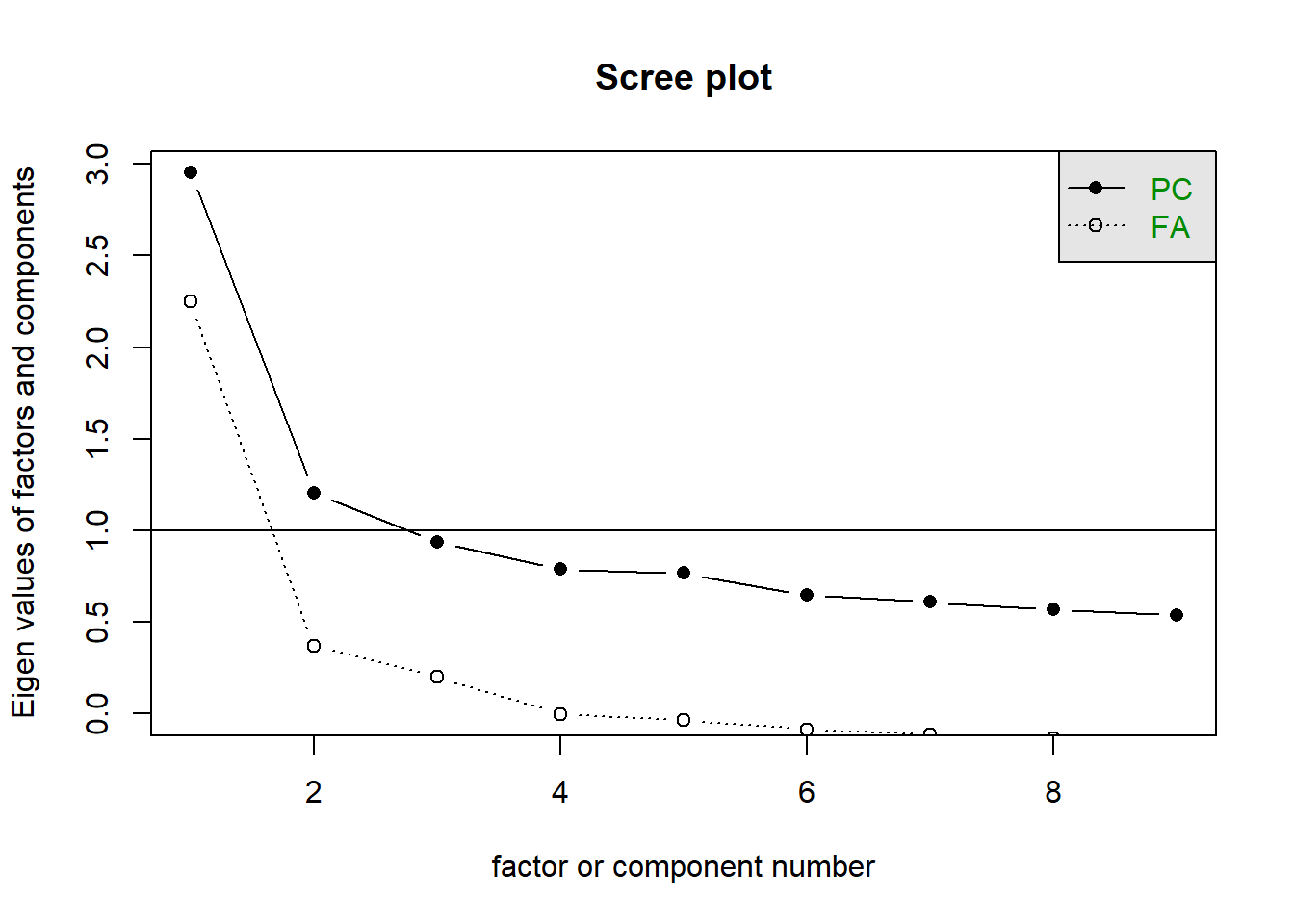
The scree plot is a plot of each factor’s eigenvalue. This method relies on visual inspection - namely, you want to identify the ‘elbow’ of the line, or the point where the graph levels off. This is the point where the amount of variance explained by additional factors reaches that diminishing returns phase.
psych will plot two sets of eigenvalues - one ‘component’-based set (which is what we calculated above), and one ‘factor’-based set (which is what Jamovi gives you).
This is inherently a bit subjective, and sometimes isn’t very clear. On our scree plot below, it looks like four factors is the point where the diminishing returns begin, so we would go with retaining four factors. However, a more conservative interpreter could reasonably argue that we should only retain 2 factors.
12.4.4 Parallel analysis
Parallel analysis (Horn, 1965) is a sophisticated technique that involves simulating random datasets of the same size as our actual dataset, and comparing our dataset’s eigenvalues against the random dataset’s eigenvalues. Parallel analysis is generally demonstrated using a scree plot with an additional scree line for the simulated datasets. The fa.parallel() function will run this for us.8
The number of factors to retain is determined by the number of factors where our actual data’s eigenvalue exceeds the simulated dataset’s eigenvalue.9 In this instance, we would choose to retain three factors, as the actual data eigenvalues clearly drop below the simulated data at four factors.
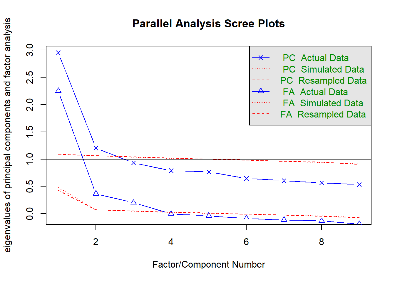
## Parallel analysis suggests that the number of factors = 3 and the number of components = 212.4.5 Velicer’s Minimum Average Partials (MAP) test
The Minimum Average Partials (MAP; Velicer, 1976) test is another powerful test that is generally useful at identifying how many factors should be extracted. It basically works by calculating the partial correlations between items and finding their average after removing the variance explained by the factors.
The EFA.dimensions package contains a series of helpful functions for running some EFA-related checks. The MAP test is included as part of the MAP() function:
##
##
## MINIMUM AVERAGE PARTIAL (MAP) TEST
##
## Number of cases = 2571##
## Number of variables = 9##
## Specified kind of correlations for this analysis: Pearson##
##
## Total Variance Explained (Initial Eigenvalues):## Eigenvalues Proportion of Variance Cumulative Prop. Variance
## Factor 1 2.95 0.33 0.33
## Factor 2 1.20 0.13 0.46
## Factor 3 0.93 0.10 0.57
## Factor 4 0.79 0.09 0.65
## Factor 5 0.77 0.09 0.74
## Factor 6 0.65 0.07 0.81
## Factor 7 0.61 0.07 0.88
## Factor 8 0.57 0.06 0.94
## Factor 9 0.54 0.06 1.00##
## Velicer's m values## root m_pr_squared m_pr_4rth_power
## 0 0.06439 0.98585
## 1 0.02330 0.12171
## 2 0.04126 0.19847
## 3 0.06469 0.32682
## 4 0.12008 1.09402
## 5 0.20155 3.03325
## 6 0.28088 4.94336
## 7 0.48302 16.87119
## 8 1.00000 91.00000##
## The smallest partial_r_squared m value is 0.0233##
## The smallest partial_r_4rth_power m value is 0.12171##
## The number of components according to the original (1976) MAP Test is = 1##
## The number of components according to the revised (2000) MAP Test is = 1Here, we look for the number of factors with the minimum average partial correlation (hence the name). There are two forms of this test, one based on the original and a revised version - the only difference is that the original looks for the average squared correlation, while the revised version calculates it to the 4th power. As we can see, the smallest average correlation in both versions occurs when we extract one factor.
12.4.6 How to decide?
Let’s summarise our interim decisions so far:
- Kaiser’s rule suggests 1 factor
- Visual scree plot inspection suggests either 2 or 4 factors
- Parallel analysis suggests 3 factors
- MAP suggests 1 factor
How do we decide what to use? Decades of empirical and simulation literature have shown a couple of things:
- Parallel analysis is one of the best methods of identifying how many factors should be retained. While it is sensitive to various things like sample size, simulation studies have shown that parallel analysis consistently outperforms other methods in terms of how many factors should be retained.
- In contrast, do not use the Kaiser rule! The Kaiser rule will consistently misestimate the number of factors - often, the misestimation will be quite severe. It is an extremely popular rule because a) it is simple to interpret and b) SPSS, which was the dominant statistical program of choice for a very long time, defaults to only using the Kaiser rule for PCA/EFA.
- Theoretical and practical considerations should also inform your decision making. If parallel analysis suggests 7 factors, for example, but those 7 factors are hard to interpret then you should probably not run with that by default. Instead, the next thing to do would be to step through solutions that remove one factor at a time until an acceptable, interpretable model has been reached.
There are other methods of identifying factors, such as Vellicer’s Minimum Average Partials test, but Jamovi does not provide these options. In the absence of any strong justification for anything else, it is best to fall back on parallel analysis. Thus, it’s best if we go with three factors.
The
EFA.dimensionspackage has a similar function calledRAWPAR().↩︎As you can see from the output, there are two ways of calculating these eigenvalues - using either a PCA or PAF (principal axis factoring). The
fa.parallel()function uses both. Although counterintuitive given that they are not the same technique conceptually, the PCA-based output (i.e. number of components) is the typical method, and actually does perform well at correctly identifying the number of factors to extract. Jamovi appears to default to PAF-based eigenvalues, however.↩︎