13.4 Moderation: Introduction

We start the second half of this module with an overview of what moderation is, and how it can be used. On the next page we will go through a worked example.

13.4.1 Refresher on interactions

If you have completed the module on factorial ANOVAs, you’ll be familiar with the concept of an interaction:

where the effect of one IV depends on the effect of another IV.

At the time we dealt with interactions between categorical predictors, i.e. variables with discrete, defined and mutually exclusive groupings in the data - e.g. sex (male, female) vs treatment (drug, placebo). We essentially estimate mean scores for each combination of categories in our data, and compare the variouos combinations on our continuous outcome measure, leading to graphs like these:

However, one thing we haven’t looked at in great detail are interaction effects between continuous predictors.

13.4.2 Moderation

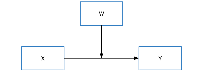
Moderation occurs when one variable influences the relationship between a predictor (X) and an outcome (Y). In contrast to a mediator, which we denote as M, we typically denote a moderator using W. Put simply, the existence of a moderator implies that the effect of X on Y depends on the value of W.

That might sound familiar… and for good reason! If you thought that just sounds like an interaction effect, you’d be absolutely right. At a statistical/mathematical level, a moderation is simply an interaction between two continuous predictors, and thus you can think of moderation and interaction as the same thing. That means that we can define a moderation using a regression formula as follows:

\[ y = \beta_0 + \beta_1x + \beta_2w + \beta_3(xw) + \epsilon_i \]

Where \(\beta_1\) and \(\beta_2\) and are regression coefficients (slopes) for X and W respectively, and \(\beta_3\) is the interaction effect.

However, you may have already clocked that this may not be as easy as it may be for a factorial ANOVA, where we deal with categorical predictors. After all, at least in the categorical instance we could group observations based on the combinations of the two predictors. For example, in a factorial ANOVA with sex as one of the variables, we could plot/test an effect between a predictor and an outcome for men and women separately. But how do we do this for continuous variables, where there are no ‘clear’ cutpoints? To unpack a moderation, there are two techniques we can apply.

13.4.3 Simple slopes

The first approach is the simple slopes approach, which is similar in principle to simple effects tests after factorial ANOVAs. The basic idea of a simple slopes test is to calculate the predicted values between X and Y, for multiple levels of the moderator W. The standard approach is to take the mean value of the moderator W, as well as 1 SD above and below the mean, and calculate the regression slopes for each level of the moderator. We can then plot this as follows:

From this graph, we can infer the nature of the interaction. In this example, for participants high on the moderator (red line), the relationship between X and Y is stronger; consequently, for participants low on the moderator (blue line), participants show a weaker relationship.

Of course, we can also choose more points, e.g. if we also wanted to look at +/- 2SD, or at percentile-based cutpoints we could do so.

13.4.4 The Johnson-Neyman technique

A critique of the simple slopes, or “pick-a-point” approach is that the selected points are relatively arbitrary. While +/- 1SD make sense as cutpoints, we tend to choose those in the absence of anything especially meaningful or precise. A second technique for probing a continuous interaction/moderation is called the Johnson-Neyman (JN) technique. The basic idea of the Johnson-Neyman technique is that it identifies the point at which the moderator no longer significantly interacts with the predictor.

The exact maths behind this is complex, but in short it aims to identify the values of W that are equal to or below a critical t value for a significant interaction effect.

We visualise the results of the Johnson-Neyman technique with a plot, which plots values of the moderator (W) on the x-axis against the slope of the predictor on the y-axis. Here’s an example (from the help docs for the interactions package in R:

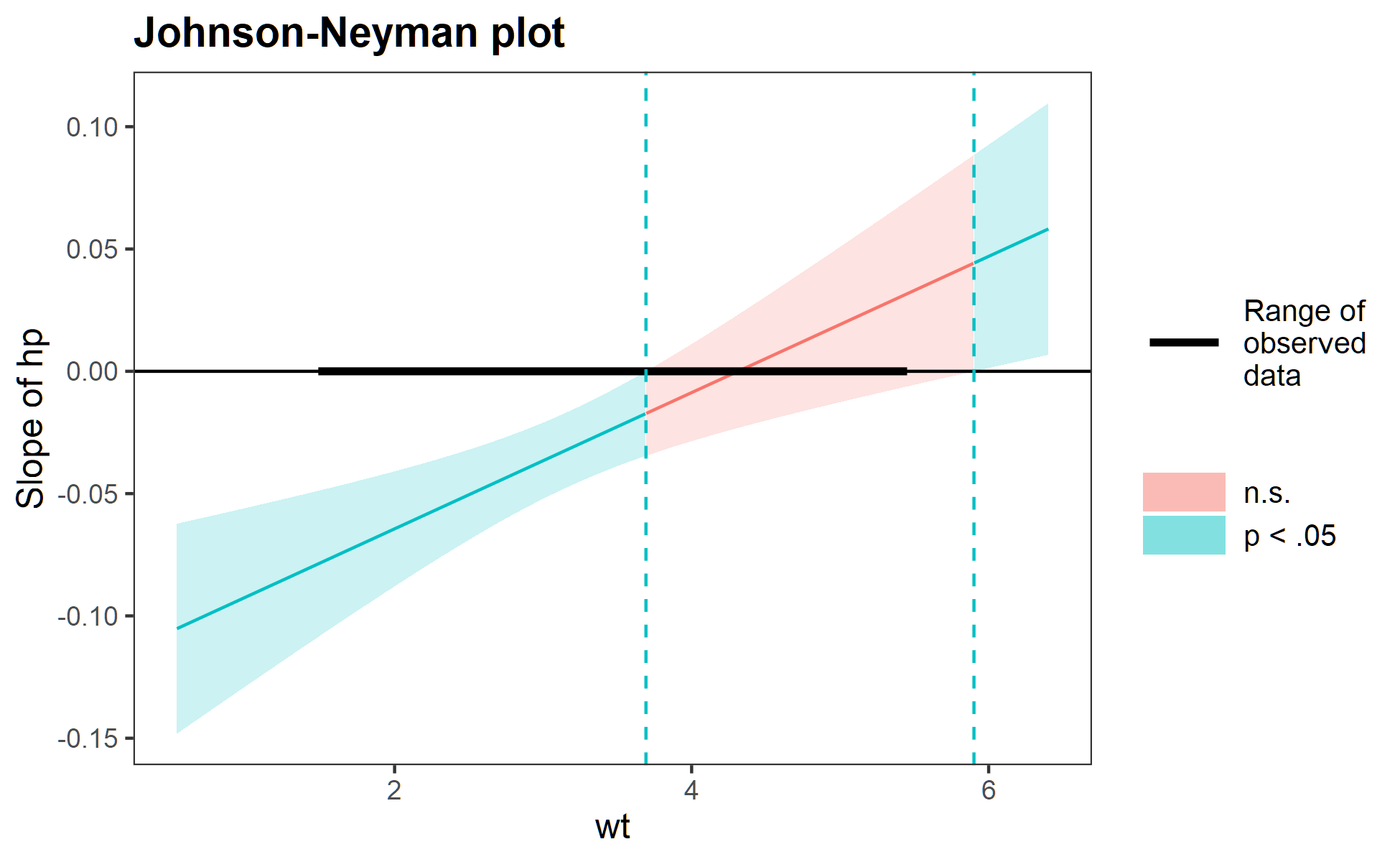
The red shaded region indicates where the moderation is non-significant. So, in this instance, values of the moderator between ~ 3.8 and 5.9 (as an eyeball guess) do not significantly moderate the relationship between the predictor and outcome. Values above or below this, however, do indicate significant moderation. Using the PROCESS macro in SPSS/R, it’s possible to get the exact values for where this range starts and ends.