3.3 Variability
The other important part of describing data is in how spread out it is. Is our data tightly bunched together, or is it very spread out? This helps us understand where most of our data falls, as well as how it looks.
3.3.1 The variability of data
The other key way of describing data is in its spread, or distribution. The way data is distributed can give key insights into how that data should be treated.
Consider the following graphs below.
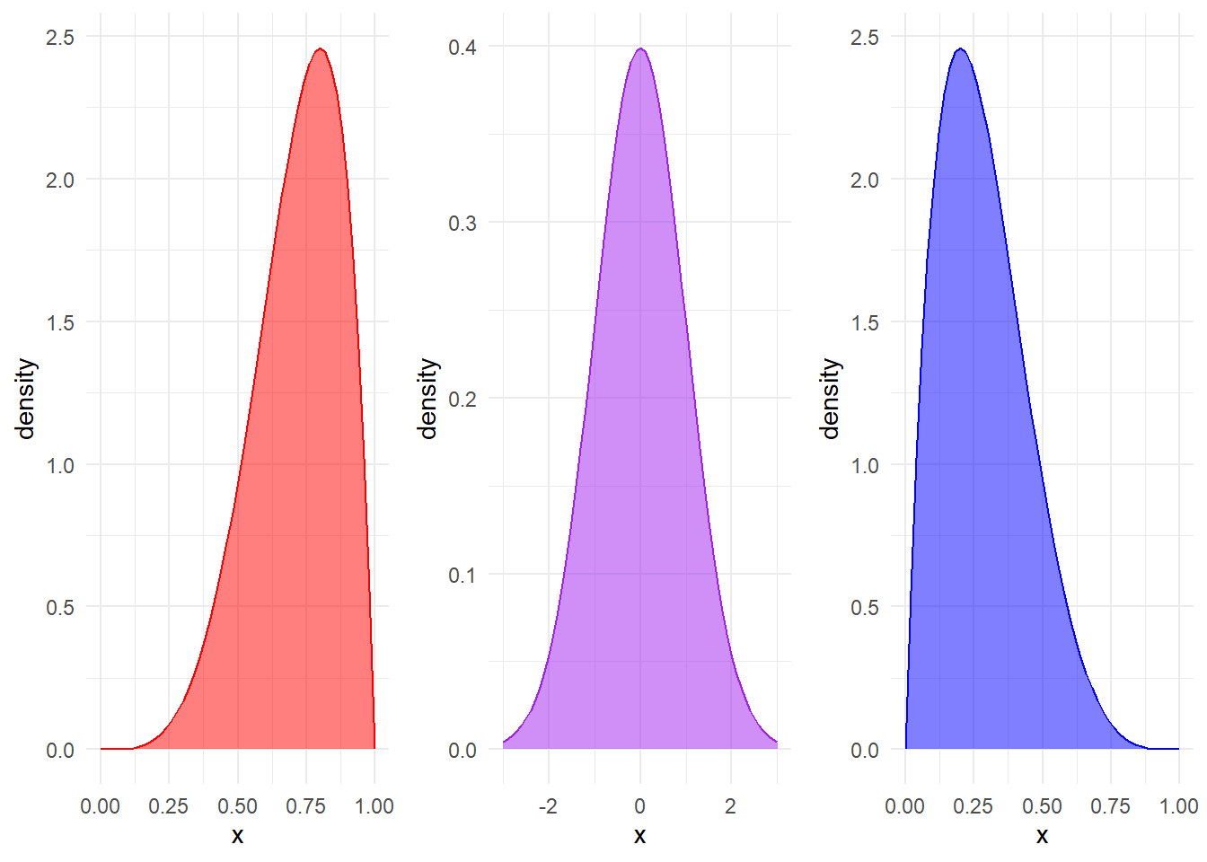
You can see that all three graphs peak at around the same point, but look very different outside of that. The orange line is narrow, while the red line is considerably more spread out. All of these graphs peak at the same point but still look very different. Therefore, they have very different spreads, or distributions.
We saw on the last page that we can quantify how far values are spread apart by finding the range. However, this isn’t always a good idea - two datasets with the exact same range can look wildly different. Therefore, we need ways of quantifying how data is spread out as well.
3.3.2 Percentiles, and the IQR
A basic way of describing variability in our dataset is by reporting percentiles or quantiles of the data. This is simply reporting what values fall within a certain percentage of the range of the data. For example, the 20th percentile captures all data that is in the bottom 20% of the sample.
Consider the following basic dataset:
## [1] 7 10 8 1 6 5 9 3 3 4 3 0 8 8 4 9 7 1 1 5You can use the quantile() function to get R to calculate percentiles for you. quantile() needs the name of a vector as the first argument, and the desired percentile as a decimal for the prob argument (e.g. 20% = 0.2).
We can, for instance, make the following statements:
- The 25th percentile is the value 3 (count five values from the left - this is 25% of the data).
- The median is 5 (the middle 2 values are 5), which is also the 50th percentile
- The 90th percentile is 9.
## 25%
## 3## 50%
## 5## 90%
## 9quantile() can return multiple percentiles by giving a vector of decimals to the prob argument. For an IQR, we can tell R to calculate percentiles for the vector c(0.25, 0.75) - representing the 25th and 75th percentiles:
## 25% 75%
##   3   8
A specific form of this that can be quite useful is the interquartile range (IQR), which describes the middle 50% of the data (i.e. 25% either side of the median). It is a single value that represents the 75th percentile score minus the 25th percentile score.
If a dataset is heavily skewed, for instance, reporting the median with the IQR can be a useful way of more accurately capturing the basic features of the data. In this instance, the IQR would be 8 - 3 = 5. You can use the IQR() function to calculate this too (note the na.rm = TRUE)).
## [1] 53.3.3 Standard deviation
Standard deviation (\(\sigma\), or SD) describes how spread out our data is within our sample, in standard (i.e. comparable) units. Data that is spread out widely (like the red curve above) will have a large standard deviation; likewise, data that has a narrow spread will have a small standard deviation. We’ll touch on this a bit more in the following pages, but for now just remember what a standard deviation is for.
To calculate standard deviation, we first calculate variance, which is another measure of spread:
\[ Variance = \frac{\Sigma (x_i - \bar{x} )^2}{n - 1} \]
Or, in human terms:
- Take each data point (\(x_i\))
- Subtract the mean from each data point (x with the bar) and square that difference
- Add them all up together
- Divide by \(n - 1\)
And then to calculate standard deviation, we simply take the square root of the variance.
\[ SD = \sqrt{Variance} \] Or, in full formula form:
\[ SD = \sqrt{\frac{\Sigma (x_i - \bar{x} )^2}{n - 1}} \]
Standard deviations (SD) should reported alongside means when results are written up (consult an APA guide).
To calculate standard deviations in R, use the sd() function. Once again, this has an na.rm argument you can specify.
## [1] 1.75119