9.3 Simple effects tests
Remember from the previous page that when we have two predictors, we end up with three model terms:
- A, a main effect
- B, a main effect
- A x B, which is our interaction effect
Therefore, we end up with two types of effects that we need to interpret: main effects, and interaction effects. An interaction effect is what we call a higher-order term, in that it is a more complex term in our model. We test the significance of each term, giving us three p-values and sets of test statistics.
Here’s an example of a two-way ANOVA with a significant interaction. Notice that there are three effects here: one for gender, one for education and the gender x education level interaction. (We’ll go through how to run these models a bit later.)
## Anova Table (Type 3 tests)
##
## Response: score
##                   Effect    df  MSE          F  pes p.value
## 1                 gender 1, 52 0.30       0.59 .011    .448
## 2        education_level 2, 52 0.30 189.17 *** .879   <.001
## 3 gender:education_level 2, 52 0.30    7.34 ** .220    .002
## ---
## Signif. codes:  0 '***' 0.001 '**' 0.01 '*' 0.05 '+' 0.1 ' ' 1
How do we interpret this? Clearly, we have no main effect of gender (p = .448) but we do have an effect of education level (p < .001). We also have a significant interaction term: gender x education (p = .002).
Here is where something called the principle of marginality kicks in. The principle of marginality, states that if two variables interact with each other, the main effects of each variable are marginal to their interaction. In more simple terms, this means that a significant interaction is a better explanation of the main effects than the main effects themselves. In context, this means that the significant effect of education level is actually best explained by decomposing the gender x education level interaction. Therefore, if you have a significant interaction you want to break this down first. If the interaction is not significant, you can run post-hocs on the main effects only.
But like a regular ANOVA, this only tells us that there is an interaction. How do we find out which means are different?
9.3.1 Simple effects tests
One option is to conduct post-hoc tests like normal, and run post-hocs on the interaction term. But this is not necessarily meaningful:
##   Tukey multiple comparisons of means
##     95% family-wise confidence level
##
## Fit: aov(formula = tmp_formula, data = dat.ret, contrasts = contrasts)
##
## $gender
##                  diff         lwr       upr     p adj
## male-female 0.1932143 -0.09680436 0.4832329 0.1870895
##
## $education_level
##                          diff       lwr        upr     p adj
## school-college     -0.7573684 -1.187898 -0.3268386 0.0002637
## university-college  2.4944417  2.069328  2.9195559 0.0000000
## university-school   3.2518102  2.826696  3.6769243 0.0000000
##
## $`gender:education_level`
##                                         diff        lwr          upr     p adj
## male:college-female:college       -0.2396667 -0.9873581  0.508024749 0.9317495
## female:school-female:college      -0.7220000 -1.4497494  0.005749384 0.0529764
## male:school-female:college        -1.0363333 -1.7840247 -0.288641918 0.0019203
## female:university-female:college   1.9430000  1.2152506  2.670749384 0.0000000
## male:university-female:college     2.8290000  2.1012506  3.556749384 0.0000000
## female:school-male:college        -0.4823333 -1.2300247  0.265358082 0.4086560
## male:school-male:college          -0.7966667 -1.5637819 -0.029551460 0.0374890
## female:university-male:college     2.1826667  1.4349753  2.930358082 0.0000000
## male:university-male:college       3.0686667  2.3209753  3.816358082 0.0000000
## male:school-female:school         -0.3143333 -1.0620247  0.433358082 0.8132166
## female:university-female:school    2.6650000  1.9372506  3.392749384 0.0000000
## male:university-female:school      3.5510000  2.8232506  4.278749384 0.0000000
## female:university-male:school      2.9793333  2.2316419  3.727024749 0.0000000
## male:university-male:school        3.8653333  3.1176419  4.613024749 0.0000000
## male:university-female:university  0.8860000  0.1582506  1.613749384 0.0087499
A more targeted approach is to conduct simple effects tests. Simple effects tests are a form of pairwise comparisons that are run to break down an interaction. It involves running pairwise comparisons between one predictor at every level of the other predictor.
Using the example above, this might include running pairwise comparisons between education levels for males and females separately:
## gender = female:
##  contrast             estimate    SE df t.ratio p.value
##  college - school        0.722 0.246 52   2.935  0.0050
##  college - university   -1.943 0.246 52  -7.899 <0.0001
##  school - university    -2.665 0.246 52 -10.834 <0.0001
##
## gender = male:
##  contrast             estimate    SE df t.ratio p.value
##  college - school        0.797 0.259 52   3.073  0.0034
##  college - university   -3.069 0.253 52 -12.143 <0.0001
##  school - university    -3.865 0.253 52 -15.295 <0.0001
Or, to spin it the other way, you might compare males and females for each education level separately:
## education_level = college:
##  contrast      estimate    SE df t.ratio p.value
##  female - male    0.240 0.253 52   0.948  0.3473
##
## education_level = school:
##  contrast      estimate    SE df t.ratio p.value
##  female - male    0.314 0.253 52   1.244  0.2191
##
## education_level = university:
##  contrast      estimate    SE df t.ratio p.value
##  female - male   -0.886 0.246 52  -3.602  0.0007
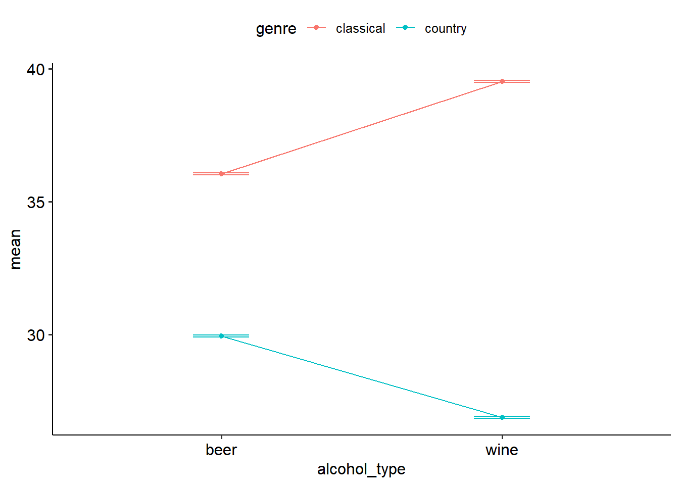
Generally, it is wise to run simple effects tests both ways - as this decomposes the interaction into something that is interpretable. This is usually guided by theoretical reasons (i.e. a hypothesis about which simple effects to run). Of course, a good graph will tell the rest of the story:
