5.2 The chi-square distribution
On the previous page we introduced the formula for a chi-square test statistic. But what do we do with it? We’ll go through this below in detail, given that this is the first time we’re coming across an actual test. While a computer will do all of this stuff automatically, it’s useful to know the actual mechanisms underlying the test.
5.2.1 The chi-square distribution
Recall from Week 6 about how hypothesis tests work - we calculate a test statistic that conforms to a particular distribution, and we assess how likely our observed test statistic is (or greater) on this distribution, assuming the null hypothesis is true. This gives us the p-value for that test. With that in mind, the chi-square distribution that underlies the chi-square test looks something like this:
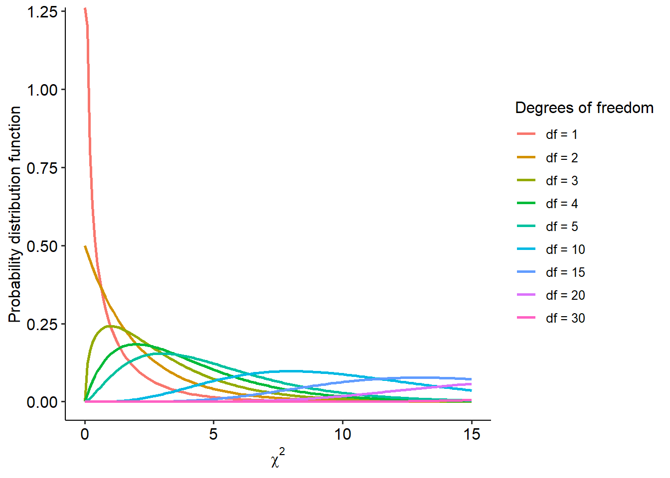
The shape of the chi-square distribution is only dependent on the degrees of freedom (df). We’ll look at how to calculate degrees of freedom for various tests, including the family of chi-square tests, as we move along the subject.
Here is the same set of lines above, but shown in their own plot this time:
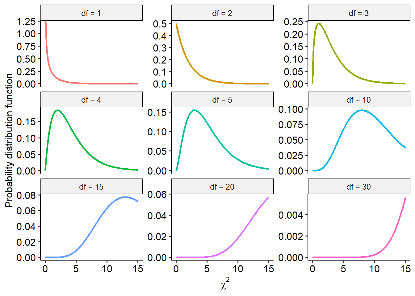
As you can hopefully see, the chi-square distribution is very heavily skewed at lower degrees of freedom (and therefore in smaller sample sizes). As degrees of freedom increase though, it approximates a normal distribution. For instance, here’s what the chi-square distribution looks like when df = 100:
5.2.2 Hypothesis testing in chi-squares
At this point, also recall that p-values are the probability that we would get our observed result (or greater), assuming the null hypothesis is true.
Here is our first application of this concept. When we use a chi-square test, we are performing the following basic steps:
- Establish null and alternative hypotheses
- Determine alpha level (in this case, \(\alpha\) = .05 as always)
- Calculate our test statistic - here, this is the chi-square statistic
- Compare our chi-square test statistic against the chi-square distribution
- Calculate how likely we would have seen our chi-square value or greater on this distribution a. Or, alternatively, establish a critical chi-square value - the value that must be crossed for a result to be significant
We’ll expand on this more in the next couple of pages.
5.2.3 Calculating significance
Let’s say that we have a df of 5. How do we know where the critical chi-square value is?
For that, we consult a chi-square table. This table gives the critical chi-square value at a set degrees of freedom and alpha level. These are freely available online, but here’s a short excerpt. To read this table:
- The far-left column lists different degrees of freedom. We need to find the row that corresponds to df = 5.
- Each column provides critical chi-squares at different alpha levels. We want to find the column that says .05.
- The number at both of these points tells us the critical chi-square value.
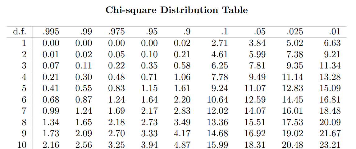
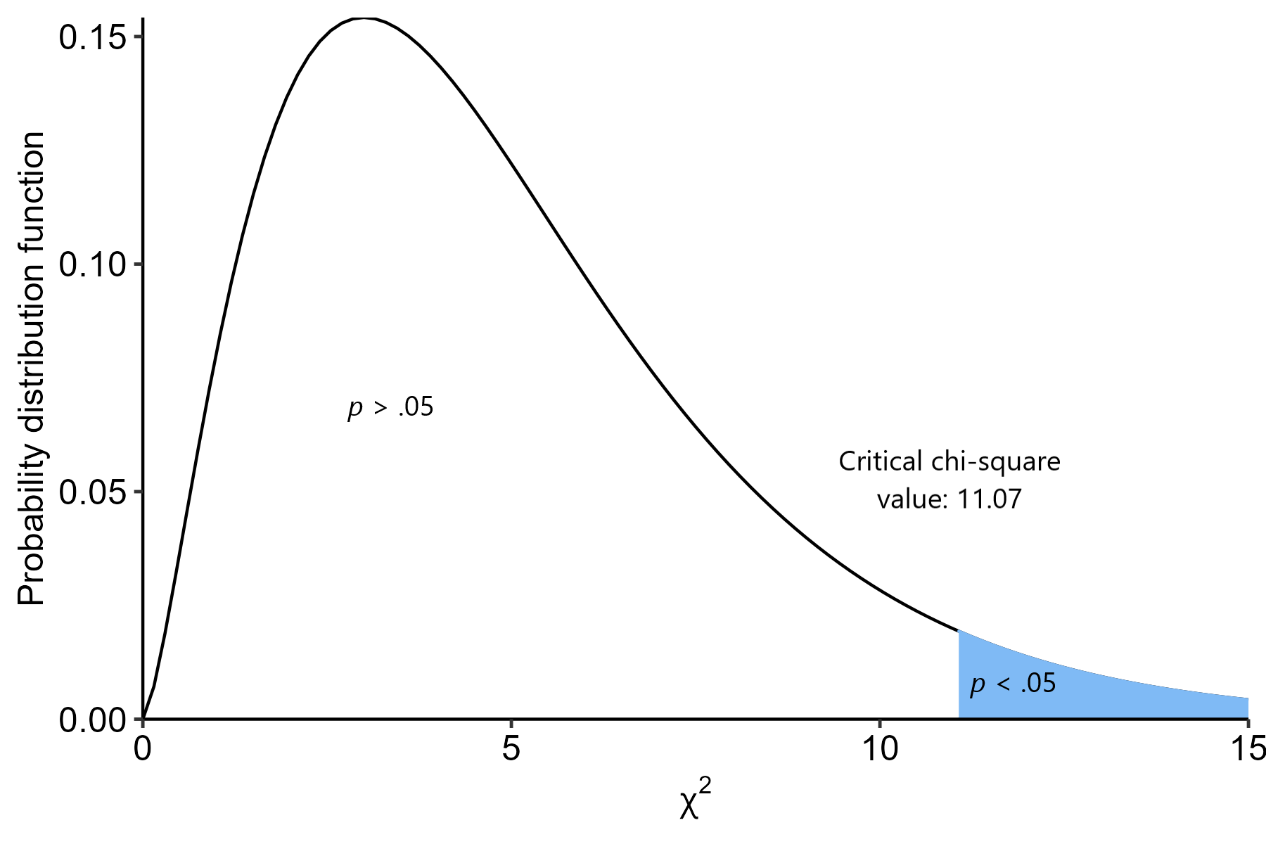
So, for a df = 5 and an \(\alpha\) = .05, the critical chi-square value is 11.07. If our own chi-square value is greater than this, the probability of that value or greater occurring (assuming the null) will be less than 5%; i.e. the boundary for statistical significance.
In picture form:
Hopefully that makes sense - this kind of logic is pretty much identical to the other tests that we will cover in the coming weeks!