C Technical details of `anova()`

## Rows: 811 Columns: 6
## ── Column specification ────────────────────────
## Delimiter: ","
## dbl (6): id, age, GoldMSI, DFS_Total, trait_anxiety, openness
## 
## ℹ Use `spec()` to retrieve the full column specification for this data.
## ℹ Specify the column types or set `show_col_types = FALSE` to quiet this message.

Technical note: this test works not too unlike a regular ANOVA, except the F-test is being conducted on the residual sums of scores. From a mathematical point of view, we are essentially conducting an F-test on the change in the residual sum of squares with the following formula:

\[ F(df_{df_b - df_a}, df_a) = \frac{MS_{comp}}{MS_{a}} = \frac{(SS_b - SS_a)/(p_a - p_b)}{SS_a/df_a} \]

Consider two models, Model A and Model B. Imagine Model B is a nested version of Model A - i.e. it it the same model as Model A but with less predictors. In our case, imagine Model B is flow_block1 (which only had one predictor) and Model A is flow_block2 (which had two). \(p_a\) is the number of coefficients in Model A including the intercept, and same with \(p_b\).

The exact process is:

Calculate the difference between residual SS in the two models - this is the \((SS_b - SS_a)\) part of the formula above. This is just the difference in RSS between model 1 (model B) and 2 (model A), i.e. 10124.2 - 9982.9 = 141.3.
Calculate the difference in df \((p_a - p_b)\). In flow_block1 we have one predictor and one intercept, so we have 2 terms - this is \(p_b\). In flow_block2 we have two predictors and one intercept, which makes \(p_a = 3\). Therefore, \((p_a - p_b) = 3 - 2 = 1\).
Calculate a mean square ratio for the comparison, which is \(MS_{comp}\). Essentially, we divide the result in step 1 (143.1) by the result in step 2 (1). This follows the same formula for mean squarews as we have seen before: \(MS = \frac{SS_{comp}}{df_{comp}}\), so \(MS_{comp} = \frac{141.3}{1} = 141.3.\) While this is identical to the sum of squares value in the table above, note that this is not the same value.
Calculate a mean square ratio between RSS and df for the new model. This is the \(SS_a/df_a\) part of the equation. \(df_a\) is calculated as \(n - p_a\), where n is the original sample size. So \(df_a = 811 - 3 = 808\). Note that the value for row 2 (which corresponds to Model A/flow_block2) under Res.df is 808.

Note that \(df_b\) is the same; \(n - p_b = 811 - 2 = 809\).

Same deal as above after that, except this time we use the values from the new model only, i.e. residual SS for model A (flow_block2) and the residual df.

\(MS_a = \frac{SS_{a}}{df_{a}}\) \(MS_a = \frac{9982.9}{808} = 12.33507\)

Calculate an F ratio between the MS of the comparison and the MS of the new model to calculate a value for F.

This is exactly the same formula as it would be for a regular ANOVA, just that now we are doing:

\[ F = \frac{MS_{comp}}{MS_{a}} \]

\(F = \frac{141.3}{12.33507} = 11.45514\)

Calculate a p-value for this F-statistic by comparing the p against an F distribution. The two dfs in the original formula are a) \(df_b - df_a\) and b) \(df_a\). Which means:

\(df_b\) is 809 - \(df_a\) is 808 = 1
\(df_a\) is 808

So we end up with a test statistic of \(F(1, 808) = 11.455\). We can use this to calculate a p-value by calculating the probability of getting a value of at least 11.455, on an F distribution with degrees of freedom parameters described above. We can visualise this below. Note that because the values for F are so infinitesimally small with these parameters and at this F-value, I’ve zoomed in the plot to visualise the highlighted area:

tibble(
  x = seq(0, 15, by = .5),
  y = df(x, df1 = 1, df2 = 809)
) %>%
  ggplot(
    aes(x = x, y = y)
  ) +
  geom_line(linewidth = 1) +
  theme_pubr() +
  geom_vline(xintercept = 11.455, linewidth = 1, colour = "royalblue") +
  annotate("text", x = 12, y = 0.0024, label = "F = 11.455") +
  stat_function(fun = df, args = list(df1 = 1, df2 = 809), 
                geom = "area", xlim = c(11.455, 15),
                fill = "royalblue", alpha = 0.5) + 
  scale_x_continuous(expand = c(0, 0), limits = c(10, NA)) + 
  scale_y_continuous(expand = c(0, 0), limits = c(0, 0.003)) +
  labs(x = "F-value", y = "Density")

## Warning: Computation failed in `stat_function()`.
## Caused by error in `fun()`:
## ! could not find function "fun"

## Warning: Removed 20 rows containing missing values or
## values outside the scale range (`geom_line()`).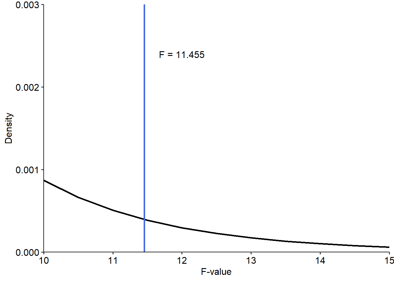

R can manually calculate a p-value with the pf() function. pf() will calculate the probability of a value on the F distribution, given the two degrees of freedom parameters to characterise the distribution. lower.tail = FALSE is used to indicate that we want to calculate the probability of getting something above our critical F-value; lower.tail = TRUE would calculuate the probability below it.

pf(11.45514, df1 = 1, df2 = 808, lower.tail = FALSE)

## [1] 0.0007473355

Note that our p-value isn’t exactly the same as the value in the table - this is because we’ve used rounded values. The code below extracts the unrounded values and uses them in the calculations. As you can see we get the exact p-value in the table.

x <- anova(flow_block1, flow_block2)
x

# Using the output from anova() to manually calculate p-value
SSb <- x$RSS[1]
SSa <- x$RSS[2]
pa <- length(coef(flow_block2))
pb <- length(coef(flow_block1))
dfa <- nrow(w10_flow) - pa
dfb <- nrow(w10_flow) - pb

f_val <- ((SSb-SSa)/(pa-pb))/(SSa/dfa)

pf(f_val, df1 = dfb-dfa, df2 = dfa, lower.tail = FALSE)

## [1] 0.0007546911

C Technical details of anova()

C Technical details of `anova()`