11.2 Theory of logistic regression
11.2.1 Introduction
All of the concepts on the previous page bring us to the main technique of this model, which is logistic regression. Logistic regression is used when we want to predict a binary outcome - for example, dead/alive status, affected/unaffected status and other scenarios where we have two primary outcomes. In this sense, we are essentially making a prediction about how likely outcome 1 is over outcome 0. Keep this in mind!
11.2.2 Modelling probabilities (sort of)
Consider the following example data. We can see that we have two columns of interest: age and outcome. Notice how outcome only takes the values of 0 and 1. This is because this is a binary variable, where 0 = one outcome and 1 = another outcome. Often, we run into situations where we are interested in predicting a binary outcome using a series of predictors, including continuous ones.
Your first thought may be to just use a simple linear regression in this instance, and sure, R isn’t going to stop you from doing so:
##
## Call:
## lm(formula = outcome ~ age, data = age_data)
##
## Residuals:
##      Min       1Q   Median       3Q      Max
## -0.36788 -0.12490  0.01528  0.13212  0.32370
##
## Coefficients:
##             Estimate Std. Error t value Pr(>|t|)
## (Intercept) -0.55739    0.16515  -3.375  0.00819 **
## age          0.10281    0.01421   7.235 4.89e-05 ***
## ---
## Signif. codes:  0 '***' 0.001 '**' 0.01 '*' 0.05 '.' 0.1 ' ' 1
##
## Residual standard error: 0.2108 on 9 degrees of freedom
## Multiple R-squared:  0.8533, Adjusted R-squared:  0.837
## F-statistic: 52.35 on 1 and 9 DF,  p-value: 4.893e-05
You might conclude that you have a significant model, with age being a significant predictor of the binary outcome. Nice! … right? Well, the moment you plot your data you may quickly see the problem with this approach:
age_data %>%
  ggplot(
    aes(x = age, y = outcome)
  ) +
  geom_point() +
  geom_smooth(method = "lm", se = FALSE)
## `geom_smooth()` using formula = 'y ~ x'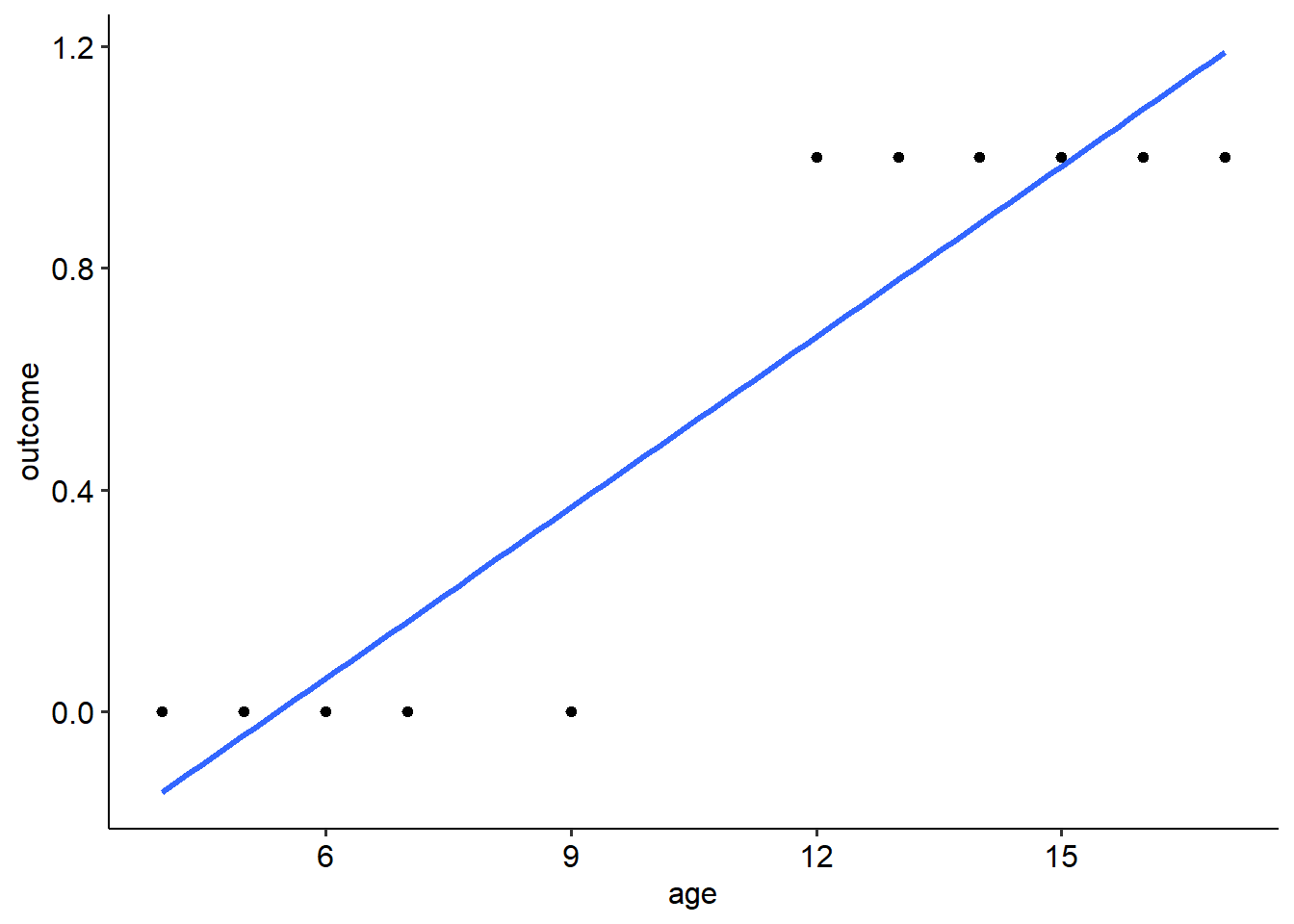
There are two huge problems here! For starters, the line currently implies that there are values that exist between 0 and 1, but what is that meant to mean? In this instance, how can we have any intermediate values between our binary outcome? The second problem is that a simple linear regression also implies that there are values that exist beyond 0 and 1, as you can hopefully see in the graph above. This also makes no sense!
11.2.3 The logistic model
In short, if we want to use our standard regression techniques, we need to model our data in a way where we can have outcomes beyond 0 or 1. Given that probabilities don’t let us do this, that’s a no-go (unless we use probit regression, but that’s a different kettle of fish). Maybe we could use the odds because they let us go past 1 - but as we saw previously, odds are bounded at a minimum of 0. However… log odds are not bounded in this way, as the log of 0 is \(- \infty\). It also turns out that with a large enough sample size, the relationship between a predictor and the log odds is linear. Therefore, we can model a regression against the log odds as follows:
\[ log(Odds) = \beta_0 + \beta_1 x_1 + \epsilon_i \] This is essentially the equation for logistic regression. We use the linear regression formula to predict the log odds of an outcome. This makes logistic regression a form of the generalised linear model (GLM). We won’t go too into GLMs beyond here, but essentially the GLM uses a linear equation to model an outcome Y using a link function. The link function describes how the predictors relate to the outcome in the model, or in other words it allows us to use a linear regression on a transformed outcome:
\[ f(Y) = \beta_0 + \beta_1 x_1 + \epsilon_i \]
In the formula above, \(f(Y)\) is used to describe the link function. In our instance, we are looking at a logit link to do a logistic regression, where our outcome is log odds (as opposed to Y, the dependent variable directly). There are many others out there that are suited for different types of data (e.g. Poisson regression). As another example of a link function, the identity function is \(f(Y) = Y\); this gives us linear regression, so really our usual regression models are just an example of the GLM.
The logistic function is characterised by a very obvious S-shaped curve:

(Technical note: the regression line that is fit is no longer least squares regression. Rather, it uses a procedure called maximum likelihood. Think of it as a different engine under the hood.)
In practice, then, this means that we can use the same kinds of thinking as we have in previous regression models to interpret logistic regression outcomes. Namely, given the formula above, a 1-unit increase in \(x_1\) will correspond to a \(\beta_1\) increase in the log odds. However, even though mathematically that makes sense, it’s hard to interpret what this actually means. What does an increase in log odds correspond to??
To solve this dilemma, we often will want to convert our outcome back into odds. To do so is simple: we simply exponentiate both sides:
\[ Odds = e^{\beta_0 + \beta_1 x_1 + \epsilon_i} \] To obtain the probability of an event occuring, we need to convert the odds back into a probability:
\[ P(Y = 1) = \frac{1}{1 + e^{-(\beta_0 + \beta_1 x_1 + \epsilon_i)}} \]