5.1 Calculating a chi-square
We’ll start this module off by briefly going through the basics of what research designs suit chi-square tests, as well as the basic maths underlying the first part of the statistical test.
5.1.1 Categorical data
As mentioned at the start of this module, chi-square tests are used when we work with categorical data - i.e., when we are dealing with counts of items or people, rather than continuous variables. Research questions focused on relationships or associations among categorical variables are suited to chi-square tests.
Every categorical variable will have levels (categories) within them. These are the different values that categorical variable can be. For example, biological sex is often coded with two levels: male and female. Or perhaps you might categorise socioeconomic status into three levels: low, medium and high bands. This is something that can form a core part of your research design. The most basic example is asking participants what their biological sex is - participants will respond with one of the two categories.
Alternatively, you can create categories from existing data. For example, many scales designed to assess psychological disorders such as depression and anxiety often have ‘cutoff’ points, where a certain score on the scale is indicative of a possible disorder. If you have everyone’s raw scores, you can convert these scores into categories depending on whether they are above or below these cutoff points (though this needs to be strongly justified).
All of this kind of data are amenable to chi-square tests, if you are interested in relationships between categorical variables. The family of chi-square tests basically work by comparing the observed values to the expected values. As the names imply, observed value simply means the number of observations we have in each category or level (i.e. what our data actually is). Expected values, on the other hand, are the number of things we would expect to see under the null hypothesis.
We can visualise categorical variables in two basic ways: a) a contingency table or b) a bar graph of counts. Below is the same set of data, shown in both forms:
5.1.2 The chi-square formula
To test whether a result is significant, remember that we need to calculate a test statistic, and see where that fits on its underlying distribution. Here, our test statistic is handily named the chi-square statistic. To calculate the chi-squared test statistic we use the following formula:
\[ \chi^2 = \Sigma \frac{(O-E)^2}{E} \]
Where:
O = observed value
E = expected value
The English translation of that above formula can be described in four steps:
Calculate observed count - expected count
Square that difference
Divide it by the expected count
Do this for each cell, and add them all up
We’ll look at this in more detail when we look at the actual tests. For the time being, here’s the key takeaway: have a look at the two graphs below, representing the observed and expected values of two different datasets.
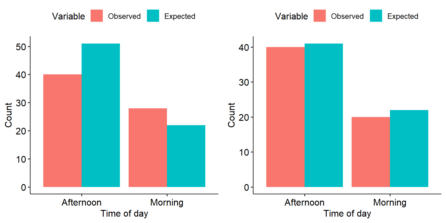
Have a think about the following:
What is each graph telling you?
The left graph appears to show noticeable differences between the observed and expected values. Based on the mathematical formula above, what will happen to the chi-square value?
Each graph represents one set of data. Based on your answers to a) and b) above, which one of the two would you expect to demonstrate a significant effect?