14.5 Kruskal-Wallis ANOVA
14.5.1 Introduction
The Kruskal-Wallis ANOVA is the non-parametric equivalent of the basic one-way ANOVA. It is essentially an extension of the Mann-Whitney U test, which has a couple of important ramifications: namely, it doesn’t assume any underlying distributions.
Like the Mann-Whitney U test, by default the Kruskal-Wallis ANOVA is purely a test of whether the data in each group come from the same underlying distributions. The KW ANOVA can only test for a difference in medians if you can assume that each group’s distribution is the same shape and spread (e.g. all groups are skewed in the same way). Otherwise, you are essentially testing for a difference in the underlying distributions.
14.5.2 Example scenario
The example data for this page and the next come from one data source, looking at language abilities in young children. These datasets contain the same participants, but the file labelled “autism_kw” takes data at one cross-section while the “autism_friedman” file contains four timepoints.
The variables in this dataset include:
- childid: Participant ID
- sicdegp: Assessment of expressive language development. Three groups: high, medium, low.
- age2: Participant’s age, centered around 2 years old. The numeric values indicate how many years have passed since the child was 2 years old.
In the "autism_friedman" dataset, the columns are labelled age_0, age_1, age_3 and age_7. These refer to the ages of 2 years old, 2yo, 5yo and 9yo respectively.- vsae: Vineland Socialisation Age Equivalent
- gender, race: Participant’s gender and race
- bestest2 - Diagnosis at age 2. Two levels: autism and PDD (pervasive developmental disorder).
We will take a look at the first autism dataset (“autism_kw”). In this dataset, we want to conduct an ANOVA comparing socialisation age equivalents (VSAE) between children with varying levels of expressive language development.
autism <- read_csv(here("data", "nonpara", "autism_long.csv")) %>%
  mutate(
    sicdegp = factor(sicdegp)
  )
## Rows: 63 Columns: 7
## ── Column specification ───────────────────────────────────
## Delimiter: ","
## chr (4): sicdegp, gender, race, bestest2
## dbl (3): childid, age2, vsae
##
## ℹ Use `spec()` to retrieve the full column specification for this data.
## ℹ Specify the column types or set `show_col_types = FALSE` to quiet this message.14.5.3 Checking assumptions (normal ANOVA)
Here’s what a regular ANOVA would look like on this data - specifically, the assumption checks. We can see that both assumptions are violated; Levene’s test is significant (F(2, 60) = 4.57, p =. 014), and the Shaprio-Wilks test is too (backed up by a funky looking Q-Q plot; W = .86, p < .001).
##
##  Shapiro-Wilk normality test
##
## data:  autism_aov$residuals
## W = 0.86118, p-value = 4.232e-06
autism_aov %>%
broom::augment() %>%
ggplot(
aes(sample = .std.resid)
) +
geom_qq() +
geom_qq_line() +
ggpubr::theme_pubr()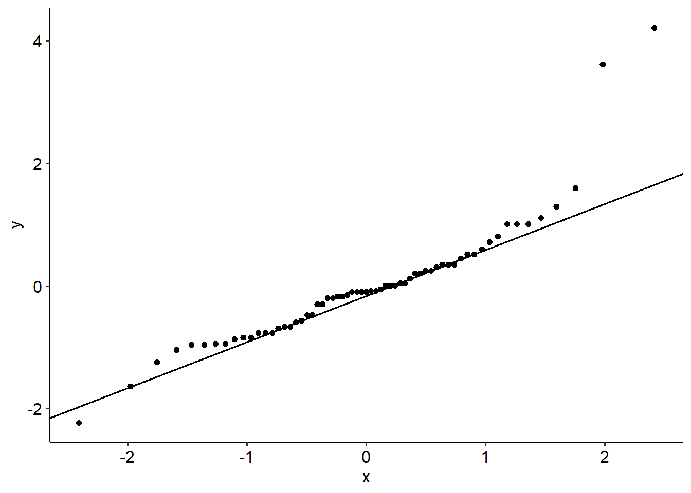
Now, these aren’t too bad in general, but let’s assume for the sake of practice that these violations are severe enough that we would consider using non-parametrics instead.
14.5.4 Output
To conduct a Kruskal-Wallis ANOVA in R, we can use the kruskal.test() function. This function works very similarly to aov(), meaning that we can provide the same notation as we normally would:
##
##  Kruskal-Wallis rank sum test
##
## data:  vsae by sicdegp
## Kruskal-Wallis chi-squared = 28.474, df = 2, p-value = 6.562e-07
Note here that the test statistic in a Kruskal-Wallis is a chi-square distribution, with a df of g - 1 (where g = number of groups). This is sometimes called H, but is mathematically equivalent to the chi-square we are familiar with. Our overall result is significant (\(\chi^2\)(2) = 28.47, p < .001).
The same notation is used for calculating effect sizes, using the rank_epsilon_squared() function from effectsize:
Here, our non-parametric effect size is epsilon squared, \(\epsilon^2\). It is not commonly seen so can be hard to interpret, but people have made various guidelines of their own.
Jamovi uses Dwass-Steel-Critchlow-Fligner tests (phew!), or simply DCSF tests, for ‘post hoc’ pairwise comparisons. We’ll use the same here for compatibility with Jamovi. The only thing you really need to know about these comparisons is that they have an in-built correction for the family-wise error rate, so do not need adjusting after the analyses have been run.
To run these tests, we need a new package called PMCMRplus. Within this package is a function called dscfAllPairsTest(), which will give us the p-values for each pairwise comparison. The required code is exactly the same as we have used above:
##
##  Pairwise comparisons using Dwass-Steele-Critchlow-Fligner all-pairs test
## data: vsae by sicdegp## high low
## low 5.4e-06 -
## med 0.0002 0.0635##
## P value adjustment method: single-stepWe can see that there is a significant difference in socialisation age between children with high versus low expressive language (p < .001), as well as between children with high versus medium expressive language (p < .001). However, there is no significant difference in socialisation age between children with low and medium expressive language (p = .064).