8.5 Linear regressions in R
Let’s now turn to an example of how to do a linear regression in R.
8.5.1 Scenario
Musical sophistication describes the various ways in which people engage with music. In general, the more ways in which people engage with music, the more musically sophisticated they are.
One hypothesis is that years of musical training will clearly influence musical sophistication. While this is a bit of a no-brainer hypothesis, we’ll test it using some example data.
## Rows: 74 Columns: 2
## ── Column specification ───────────────────────────────────
## Delimiter: ","
## dbl (2): years_training, GoldMSI
##
## ℹ Use `spec()` to retrieve the full column specification for this data.
## ℹ Specify the column types or set `show_col_types = FALSE` to quiet this message.
# This extra code is here for later
w10_goldmsi <- w10_goldmsi %>%
mutate(
id = seq(1, nrow(w10_goldmsi))
)
head(w10_goldmsi)8.5.2 Assumptions
In R the linear regression needs to be coded first before testing assumptions. Linear regression models can be built using lm(), and the same formula notation used in aov():
Let’s test our assumptions from the previous page.
Linearity: a simple scatterplot tells us that our data probably is suitable for a linear regression:
Independence: our DW test is significant (p = .021), but our test statistic is 1.54. So, even though it’s still significant it probably isn’t much of a problem.6
##
##  Durbin-Watson test
##
## data:  w10_goldmsi_lm
## DW = 1.5409, p-value = 0.02123
## alternative hypothesis: true autocorrelation is greater than 0
Homoscedasticity: To plot a residual vs fitted plot in R, there are two ways:
- plot(model, which = 1).
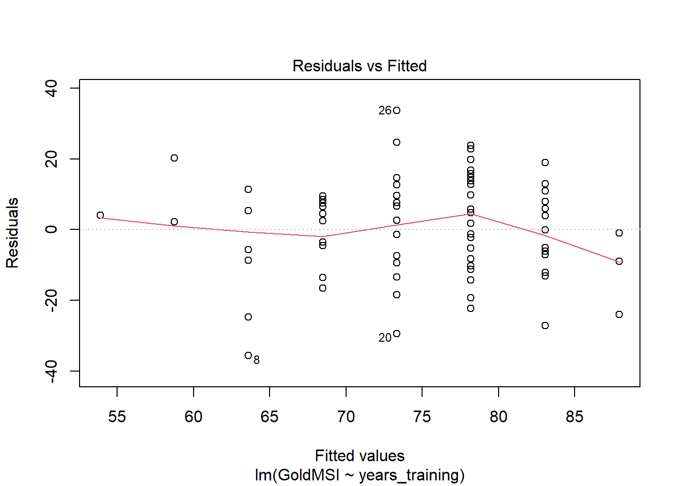
- Using ggplot, but giving the model name instead of the data and setting the x and y aesthetics as follows:
## Warning: `fortify(<lm>)` was deprecated in ggplot2 4.0.0.
## ℹ Please use `broom::augment(<lm>)` instead.
## ℹ The deprecated feature was likely used in the ggplot2
##   package.
##   Please report the issue at
##   <https://github.com/tidyverse/ggplot2/issues>.
## This warning is displayed once per session.
## Call `lifecycle::last_lifecycle_warnings()` to see where
## this warning was generated.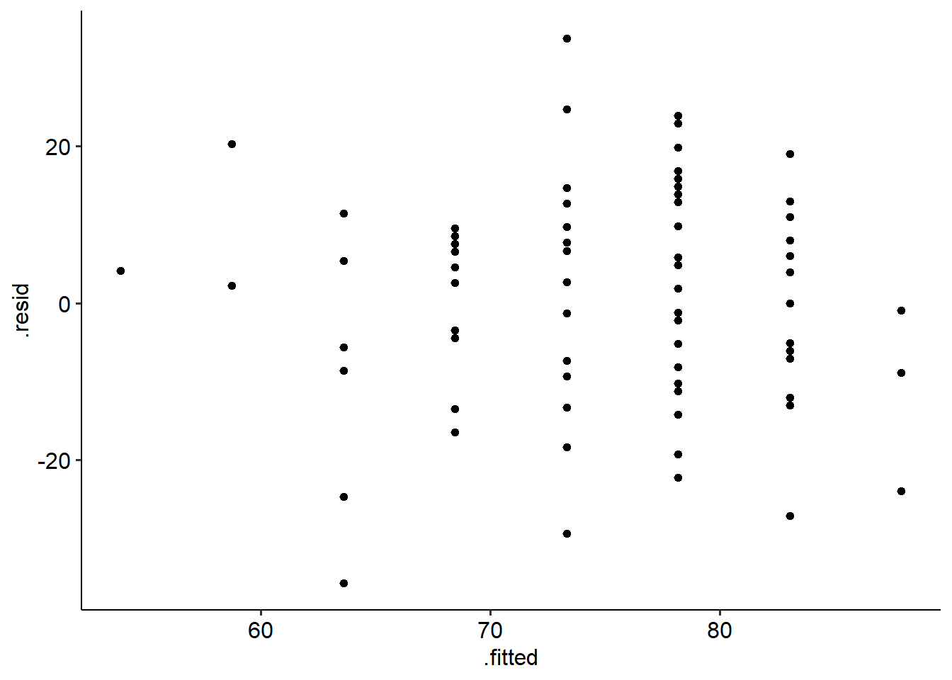
Normality of residuals: Like aov models, you can access the residuals from a given lm() model, by using the name of the lm object, followed by $residuals. This is useful for doing e.g. a Shapiro-Wilks test on the residuals, or a Q-Q plot of residuals:
##
##  Shapiro-Wilk normality test
##
## data:  w10_goldmsi_lm$residuals
## W = 0.98995, p-value = 0.8289
Our SW test is non-significant and our Q-Q plot looks ok, so this assumption is not violated.
8.5.3 Output
The output that R gives us for a linear regression comes in two parts: a test of the overall model, and a breakdown of the predictors and their slopes.
##
## Call:
## lm(formula = GoldMSI ~ years_training, data = w10_goldmsi)
##
## Residuals:
##     Min      1Q  Median      3Q     Max
## -35.617  -9.227   2.025   9.773  33.666
##
## Coefficients:
##                Estimate Std. Error t value Pr(>|t|)
## (Intercept)      53.901      5.233  10.300 8.33e-16 ***
## years_training    4.858      1.138   4.271 5.86e-05 ***
## ---
## Signif. codes:  0 '***' 0.001 '**' 0.01 '*' 0.05 '.' 0.1 ' ' 1
##
## Residual standard error: 14.61 on 72 degrees of freedom
## Multiple R-squared:  0.2021, Adjusted R-squared:  0.191
## F-statistic: 18.24 on 1 and 72 DF,  p-value: 5.859e-05
Let’s start with the overall model. This tells us whether the regression model as a whole is significant. A couple of things to note here.
- \(R^2\) is called the coefficient of determination. This value tells how much variance in the outcome is explained by the predictor. Our value is .202, which means that 20.2% of the variance in Gold-MSI scores is explained by years of training.
- The overall model test is essentially an ANOVA (we won’t go too deep into why just yet!), which tells us whether the model is significant. In this case, it is (F(1, 72) = 18.24, p < .001).
Now we can look at the middle of the output, which gives the model coefficients. This part of the output tells us whether the predictors are significant. (Given the overall model is, with one predictor we’d expect this to be significant as well!).
The Estimate column gives us the B coefficient, which is our slope. This tells us how much our outcome increases when our predictor increases by 1 unit.
From this, we can see that years of training is a significant predictor of Gold-MSI scores (t = 4.27, p < .001); for every year of training, Gold-MSI scores increase by 4.86 (given by the value under Estimate, next to our predictor variable).
Finally, we can use the confint function to return 95% confidence intervals on each regression slope:
##                   2.5 %    97.5 %
## (Intercept)    43.46925 64.332391
## years_training  2.59058  7.125814
Therefore, the 95% CI around the estimated regression coefficient of 4.86 is [2.59, 7.13].
Here is how we can write up these results. Note that for a regression, it is important to discuss both the overall model fit and the specific effect of the predictor.
We conducted a simple linear regression to examine whether years of training predicted Gold-MSI scores. The overall model was significant (F(1, 72) = 18.24, p < .001), with years of training explaining 20.2% of the variance in Gold-MSI scores (\(R^2\) = .202). Years of training was a significant positive predictor of Gold-MSI scores (B = 4.86, t = 4.27, p < .001).
Given that this data was randomly generated, it probably is due to a simulation outlier more than anything.↩︎