6.1 t-tests and the t-distribution
We begin this week’s module in much the same way we went through last week’s. We’ll look at the shape of the underlying distribution, and what determines the shape of that distribution. On this page we’ll also go through what the basic premise of the t-test is.
6.1.1 What is a t-test?
The family of t-tests, broadly speaking, are used when we want to compare one mean against another. This can take on three major forms, which we will go into later in the module:
- Is this sample mean different from the population mean?
- Are these two group means different?
- Is the mean at point 1 different to the mean at point 2?
All of these instances require a comparison between two means, which the t-tests will allow you to test for. So, in a general sense our hypotheses would be something like:
- \(H_0\): The means between the two groups are not significantly different. (i.e. \(\mu_1 = \mu_2\))
- \(H_1\): The means between the two groups are significantly different. (i.e. \(\mu_1 \neq \mu_2\))
The question of when t-tests should be used is hopefully somewhat obvious - in general, we use them we want to compare two means with each other. The important part is what kind of means they are:
- If we compare one sample mean to a hypothesised population mean, this is a one-sample t-test
- If we compare two group means, this is an independent samples t-test
- If we measure one group twice and compare the two means, this is a paired-samples t-test.
In this module, we’ll go through all three (but will emphasise the latter two especially as they see the most use).
6.1.2 The t-statistic
Last week we introduced the chi-square statistic, which is the value that we use when we want to assess whether a result is significant. When we want to assess whether a difference between two means is significant we calculate a different test statistic, which (as the name implies) is the t-statistic. While you won’t be required to calculate this by hand this week, it would be good to wrap your head around the below formula so you understand how it works in principle:
\[ t = \frac{M_1 - M_2}{SE} \]
This is how t is calculated conceptually - it is the difference in the two means over the standard error of the mean. Note that the world conceptually is stressed here because the actual formula is slightly different for each t-test, but all work on this above principle. Again, we won’t go through the maths of this in detail - this is beyond the scope of the subject!
6.1.3 The t-distribution
By now, hopefully you’re comfortable with the idea that we use our test statistic and find its position on its underlying probability distribution in order to calculate the p-value. The underlying distribution of this test is the t-distribution, which is depicted below. Note that like the chi-square distribution, degrees of freedom is the only parameter that determines its shape:
## Warning: Using `size` aesthetic for lines was deprecated in ggplot2
## 3.4.0.
## ℹ Please use `linewidth` instead.
## This warning is displayed once per session.
## Call `lifecycle::last_lifecycle_warnings()` to see where
## this warning was generated.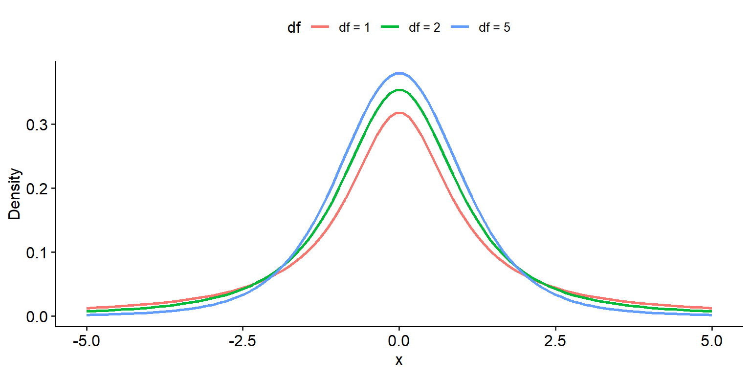
The one key difference between the t-distribution and the chi-square distribution from a mathematical point of view is that the t-distribution is symmetrical, much like the normal distribution (although they are not the same). Therefore, it is possible to get a negative t-test statistic; however, this simply reflects the order in which the groups are being compared. E.g.
- Say that Group 1 - Group 2 gives a test statistic of t = 1.5.
- If you were to enter the groups as Group 2 - Group 1 instead, the t would be -1.5. This simply reflects the ordering of the groups.
6.1.4 The t-table
Once again, like the chi-square we have a beautiful little table for calculating a critical t-value. We won’t go into too much depth over how this works because it works exactly like how it does for chi-squares - find the row corresponding to your degrees of freedom, then find the column corresponding to your alpha level.
Yes, there are a lot of cross-references to what we covered last week with chi-squares - and that’s a good thing! The point here is that conceptually, the process of testing hypotheses using t-tests is exactly the same as what we did with chi-squares, but the specific design and maths are different.