7.6 One-way repeated measures ANOVA
The second form of ANOVA that we will cover in this module is the repeated measures ANOVA (sometimes abbreviated as RM-ANOVA). While it shares many features with the basic one-way ANOVA, the nature of repeated measures data introduces some key differences in the interpretation and calculation of this test.
7.6.1 Repeated measures ANOVAs
In principle, a repeated-measures ANOVA is very similar to the paired-samples t-test: both are repeated measures versions of their respective between-groups versions. So naturally, repeated-measures ANOVAs are used when we test one sample two or more times (again, like a regular ANOVA, it’s typically for 3+ times but can be used for two).
It shares many similarities with the basic one-way ANOVA, albeit with one additional step in calculation: because we now test the same sample repeatedly, we need to account for variance within subjects. We won’t go too into detail about how that’s calculated here, but essentially we split within-groups variance into subject variance and error/residual variance. This essentially adds an extra step to the ANOVA table.
7.6.2 Example data
In this example, we’ll use a dataset derived from McPherson (2005). This is a subset of data where children were scored on their ability to play songs from memory over three years - 1997 - 1999. We’re interested in seeing whether this change over time is significant - therefore, time (3 levels) is our independent variable, while playing from memory is our dependent variable.
## Rows: 95 Columns: 4
## ── Column specification ───────────────────────────────────
## Delimiter: ","
## dbl (4): Participant, PFM_97, PFM_98, PFM_99
##
## ℹ Use `spec()` to retrieve the full column specification for this data.
## ℹ Specify the column types or set `show_col_types = FALSE` to quiet this message.For further analyses, we’ll shape this into long format:
7.6.3 Assumption checks
There are two main assumptions for a repeated-measures ANOVA. Note that while the independence assumption as we know it doesn’t apply here (by definition, repeated data is dependent), good experimental design should still aim to ensure that participants are independent of each other.
- The residuals should be normally distributed.
Our usual tests apply here too. Below is a QQ plot, which might suggest that our residuals aren’t normally distributed. (Use the data and perform a SW test on it to see what happens!)
aov(memory_score ~ time, data = w9_memory) %>%
  broom::augment() %>%
  ggplot(aes(sample = .std.resid)) +
  geom_qq() +
  geom_qq_line()
## Warning: The `augment()` method for objects of class `aov` is not maintained by the broom team, and is only supported through the `lm` tidier method. Please be cautious in interpreting and reporting broom output.
##
## This warning is displayed once per session.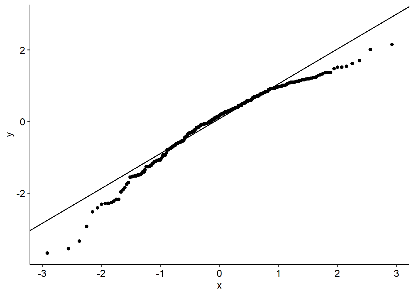
- The sphericity assumption. Sphericity is assumed if, the variances of the differences between each level of the IV are equal. Think of it as a form of the equality of variances assumption, where we assumed that the variances within groups were equal. The sphericity assumption applies to the differences between T1 and T2, then T2 and T3… etc etc.
Note that sphericity only applies when you have at least 3 levels of your IV (i.e. 3 timepoints). We can formally test it using Mauchly’s test of sphericity. If sphericity is violated, it means that our degrees of freedom are too high for the data, which inflates the Type I error rate.
What next? We need to apply a correction to the omnibus ANOVA, which will alter the p-value. There are two on offer: Greenhouse-Geisser and Huynh-Feldt corrections. To help decide which one to use, R also calculates a value called epsilon (\(\epsilon\)). Epsilon, in short, is a measure of sphericity; if sphericity is assumed, \(\epsilon\) = 1. If \(\epsilon\) is below 1, sphericity is violated; the smaller it is, the greater the violation and therefore the greater the correction needs to be. Therefore, these corrections alter the degrees of freedom for each test to account for this higher error rate.
(Mathematical note; the corrected dfs are calculated by multiplying the original dfs by \(\epsilon\). So e.g. if your original df is 10 and \(\epsilon\) = 0.9, your new corrected df will be 9.)
Broadly:
- If epsilon (\(\epsilon\)) > .75, use the Huynh-Feldt correction.
- If epsilon (\(\epsilon\)) < .75, use the Greenhouse-Geisser correction.
In R, most main packages will test the sphericity assumption along with the main ANOVA, so we will see this below.
7.6.4 ANOVA output
R-Note: Repeated measures ANOVAs in R are not trivial in the slightest, and adapting this was a genuine challenge. To some extent this probably reflects the differences in approach between point-and-click software compared to actually having to code the ANOVA model: the former is easy but you perhaps make many assumptions about what’s going on along the way.
For that reason, now is a good time to introduce the afex package, which stands for “analysis of factorial experiments”. The aov_ez() function will let us specify a repeated measures ANOVA in a very easy way. See below for an alternative using rstatix, although this is less flexible than the afex version.
At a minimum, you must give the following arguments to aov_ez():
id: The name of the column that identifies each participantdv: The dependent variable/outcomedata: The name of the datasetwithin: The name of the within-subjects IV/predictor
## Loading required package: lme4## Loading required package: Matrix##
## Attaching package: 'Matrix'## The following objects are masked from 'package:tidyr':
##
## expand, pack, unpack## Registered S3 method overwritten by 'lme4':
## method from
## na.action.merMod car## ************
## Welcome to afex. For support visit: http://afex.singmann.science/## - Functions for ANOVAs: aov_car(), aov_ez(), and aov_4()
## - Methods for calculating p-values with mixed(): 'S', 'KR', 'LRT', and 'PB'
## - 'afex_aov' and 'mixed' objects can be passed to emmeans() for follow-up tests
## - Get and set global package options with: afex_options()
## - Set sum-to-zero contrasts globally: set_sum_contrasts()
## - For example analyses see: browseVignettes("afex")
## ************##
## Attaching package: 'afex'## The following object is masked from 'package:lme4':
##
## lmerw9_memory_aov <- aov_ez(
id = "Participant",
dv = "memory_score",
data = w9_memory,
within = "time",
type = 3,
anova_table = list(
correction = "HF",
es = "pes"
)
)Also worth noting is the anova_table argument, which specifies options for the main output. This argument takes a list() as the argument, and we can set multiple options within this list. Here, we have set two:
correction = "HF"specifies Huynh-Felt corrections. We can also ask for Greenhouse-Geisser corrections usingcorrection = "GG".es = "pes"specifies partial eta-squared for effect size. This is ok for a one-way ANOVA; recall that for a one-way setting, normal and partial eta-squared are the same.
Now that we’ve built our ANOVA model we can ask for the output like so. This will also print out the sphericity test.
Here’s our overall output from the ANOVA. It looks (and reads) pretty much the same as our previous example, albeit with some minor differences.
To see the full output, including the sphericity test, call summary() on your ANOVA object:
##
## Univariate Type III Repeated-Measures ANOVA Assuming Sphericity
##
##              Sum Sq num Df Error SS den Df F value    Pr(>F)
## (Intercept) 3490869      1   259027     94 1266.83 < 2.2e-16 ***
## time          98948      2    70130    188  132.63 < 2.2e-16 ***
## ---
## Signif. codes:  0 '***' 0.001 '**' 0.01 '*' 0.05 '.' 0.1 ' ' 1
##
##
## Mauchly Tests for Sphericity
##
##      Test statistic  p-value
## time        0.93912 0.053894
##
##
## Greenhouse-Geisser and Huynh-Feldt Corrections
##  for Departure from Sphericity
##
##       GG eps Pr(>F[GG])
## time 0.94261  < 2.2e-16 ***
## ---
## Signif. codes:  0 '***' 0.001 '**' 0.01 '*' 0.05 '.' 0.1 ' ' 1
##
##         HF eps   Pr(>F[HF])
## time 0.9612827 2.447568e-35
Here, our p-value for Mauchly’s test is almost significant (p = .054); rather than going by a strict arbitrary cutoff, let’s assume that it has been violated (both for teaching and for methodological purposes). Here, our epsilon value is high (~.95), so let’s apply the Hyunh-Feldt correction. The associated epsilon value is \(\epsilon = .943\); when reporting the repeated measures ANOVA we need to look at the rows corresponding to the Huynh-Feldt correction.
afex will print out the corrected version of the test if you just print the object without using summary().
## Anova Table (Type 3 tests)
##
## Response: memory_score
##   Effect           df    MSE          F  pes p.value
## 1   time 1.92, 180.72 388.06 132.63 *** .585   <.001
## ---
## Signif. codes:  0 '***' 0.001 '**' 0.01 '*' 0.05 '+' 0.1 ' ' 1
##
## Sphericity correction method: HF
Thus, with the corrected output we can see our effect of time is significant (F(1.92, 180.72) = 132.63, p < .001).
A benefit of doing a repeated-measures ANOVA this way is that this model is compatible with the effectsize functions, including eta_squared():
7.6.5 Post-hoc tests
As per usual, we follow up a significant overall ANOVA with a series of post-hoc comparisons:
##  contrast        estimate   SE df lower.CL upper.CL t.ratio p.value
##  PFM_97 - PFM_98    -29.6 2.82 94    -36.5   -22.74 -10.501 <0.0001
##  PFM_97 - PFM_99    -44.9 3.08 94    -52.4   -37.38 -14.577 <0.0001
##  PFM_98 - PFM_99    -15.3 2.48 94    -21.3    -9.24  -6.170 <0.0001
##
## Confidence level used: 0.95
## Conf-level adjustment: bonferroni method for 3 estimates
## P value adjustment: holm method for 3 tests
As an alternative, we can use pairwise.t.test(). Note this time we set paired = TRUE.
##
##  Pairwise comparisons using paired t tests
##
## data:  w9_memory$memory_score and w9_memory$time
##
##        PFM_97  PFM_98
## PFM_98 < 2e-16 -
## PFM_99 < 2e-16 1.7e-08
##
## P value adjustment method: holm
From this, we can see that all three means are significantly different from each other (p < .001, for brevity’s sake). Scores increased year on year, i.e. 1997 < 1998 < 1999.
A one-way repeated measures ANOVA was conducted to examine whether scores for playing songs from memory changed over three years. We applied Huynh-Feldt corrections to account for non-sphericity. There was a significant large effect of year on performance scores (F(1.92, 180.72) = 132.63, p < .001, \(\eta^2\) = .231). Post-hoc tests with Tukey HSD corrections showed that participants scored higher in 1998 than in 1997 (mean difference, MD = 29.61, p < .001). Participants also scored higher in 1999 compared to 1998 (MD = 15.27, p < .001) and 1997 (MD = 44.88, p < .001).
7.6.6 Alternative using rstatix
As mentioned above, repeated measures ANOVAs in R are not trivial at all. The solution using rstatix above is good, although it is not fully ideal.
Below is an alternative way of running a repeated measures ANOVA, this time using the rstatix package. It even uses similar arguments to the afex version above.
## ANOVA Table (type III tests)
##
## $ANOVA
##   Effect DFn DFd       F        p p<.05   ges
## 1   time   2 188 132.625 1.19e-36     * 0.231
##
## $`Mauchly's Test for Sphericity`
##   Effect     W     p p<.05
## 1   time 0.939 0.054
##
## $`Sphericity Corrections`
##   Effect   GGe       DF[GG]    p[GG] p[GG]<.05   HFe       DF[HF]    p[HF]
## 1   time 0.943 1.89, 177.21 1.05e-34         * 0.961 1.92, 180.72 2.45e-35
##   p[HF]<.05
## 1         *
The two columns to look for are the ones labelled DF[HF] - this gives the adjusted degrees of freedom with the Huynh-Feldt corrections (DF[GG] would give Greenhouse-Geisser dfs) - and p[HF], which gives the adjusted p-value.
Note that the rstatix version is not compatible with either eta_squared() (from the effectsize package) or emmeans. If you want post-hocs, you will need to use the pairwise.t.test() function or its rstatix equivalent. However, this does mean that it is not possible to do Tukey adjustments.