10.4 Outliers

Up until this point, we’ve largely worked without considering outliers in our data. Outliers, however, are important for any and all analyses that we do, because they have an impact on our statistics.

An intuitive reason is simply because of the fact that many of our statistics involve differences between means - such as t-tests and ANOVAs - and means are susceptible to outliers. Consider the following set of values:

vector_b <- c(1, 3, 2, 4, 2)

If we take a mean, this is fairly straightforward:

mean(vector_b)

## [1] 2.4

However, imagine we have an outlier in one of our datapoints:

vector_b <- c(1, 3, 2, 50, 2)
mean(vector_b)

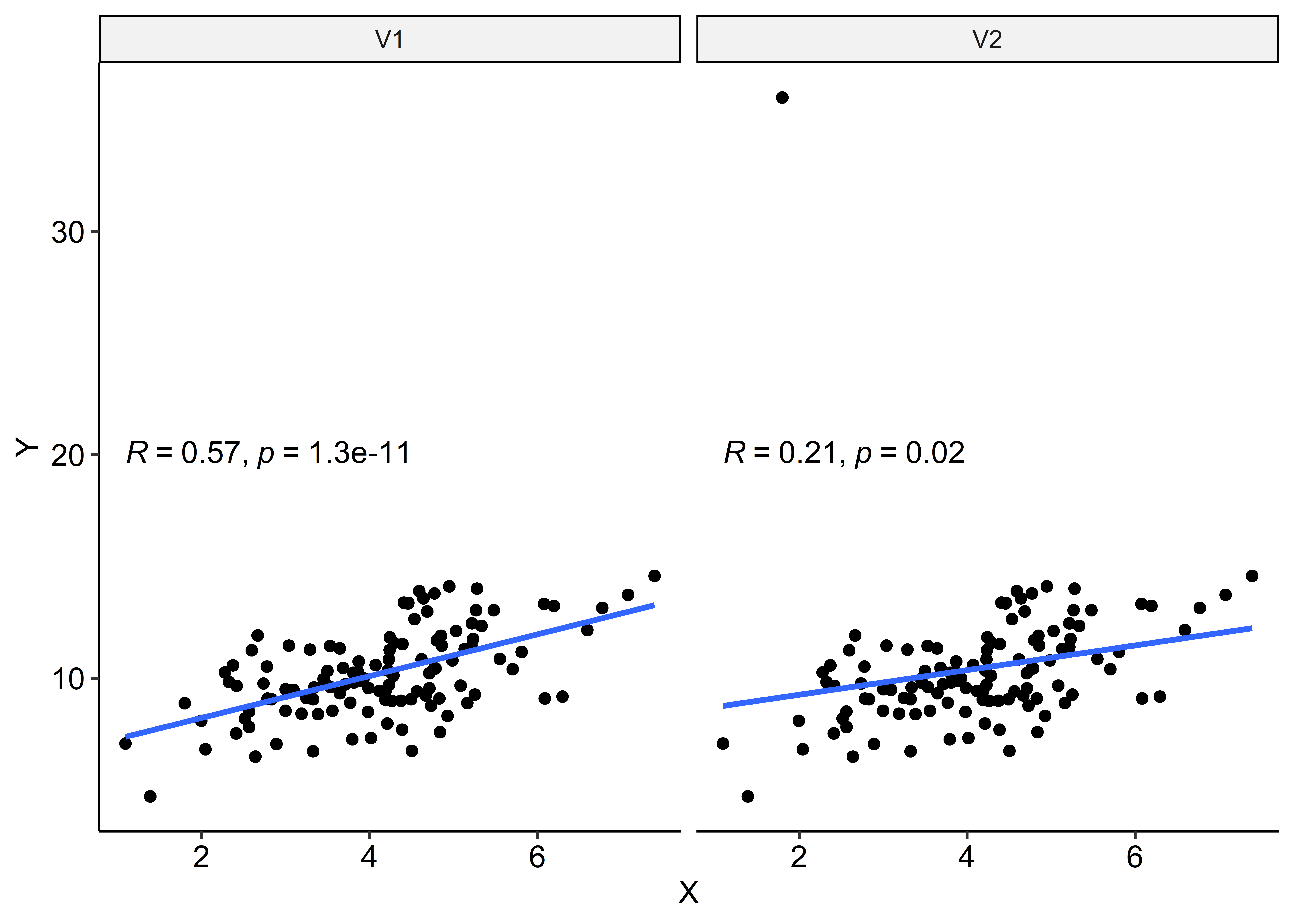
## [1] 11.6

Our estimate is now wildly different due to this outlier. Here’s another visualisation of this effect at play, with a simple regression model:

You can see that in the graph on the left, there are no visible outliers, while the graph on the right has a very clear outlier (the dot at the very top). The resulting estimate of the correlation is vastly different - r = .57 without the outlier, vs r = .21 with it included!

In short, outliers have the potential to distort our estimates. Therefore, being able to systematically identify outliers and handle them is an important step in any analysis.

Although outliers are worth considering across all types of analyses, we’ll only consider them in context of regression models here for parity with Jamovi.

Aside from visual inspection, we have two main methods of identifying outliers in our regression models. For both examples, we will use flow_block3 from the previous page.

10.4.1 Cook’s distance

Cook’s distances are a method for identifying influential points in a regression model. The basic rationale is that if a point is highly influential, it has a large effect in shaping the overall parameter estimates in the regression model. Thus, points with high Cook’s distances values are worth looking into.

Cook’s distances can be easily calculated using the cooks.distance() function in base R. You just need to spply the name of the regression model (created using lm()):

flow_cooksd <- cooks.distance(flow_block3)

This returns a singular vector of Cook’s distance values. We can then perform basic descriptives on this variable to get a sense of the range of Cook’s distance values:

mean(flow_cooksd)

## [1] 0.001356221

sd(flow_cooksd)

## [1] 0.00316087

median(flow_cooksd)

## [1] 0.0004290943

min(flow_cooksd)

## [1] 5.657846e-10

max(flow_cooksd)

## [1] 0.05169864

If you prefer a tidyverse implementation, you can use the augment() function from the broom package. This returns a whole range of values, including fitted values, residuals (both of which are useful for Q-Q plots) and Cook’s distances:

library(broom)
flow_extra <- augment(flow_block3)

flow_extra

The Cook’s distances are contained in the .cooksd column - note the full stop in front of the name is part of the column name.

As this returns a dataframe, we can then use normal tidyverse functions to wrangle this like any other dataframe.

flow_extra %>%
  summarise(
    mean = mean(.cooksd),
    sd = sd(.cooksd),
    median = median(.cooksd),
    min = min(.cooksd),
    max = max(.cooksd)
  )

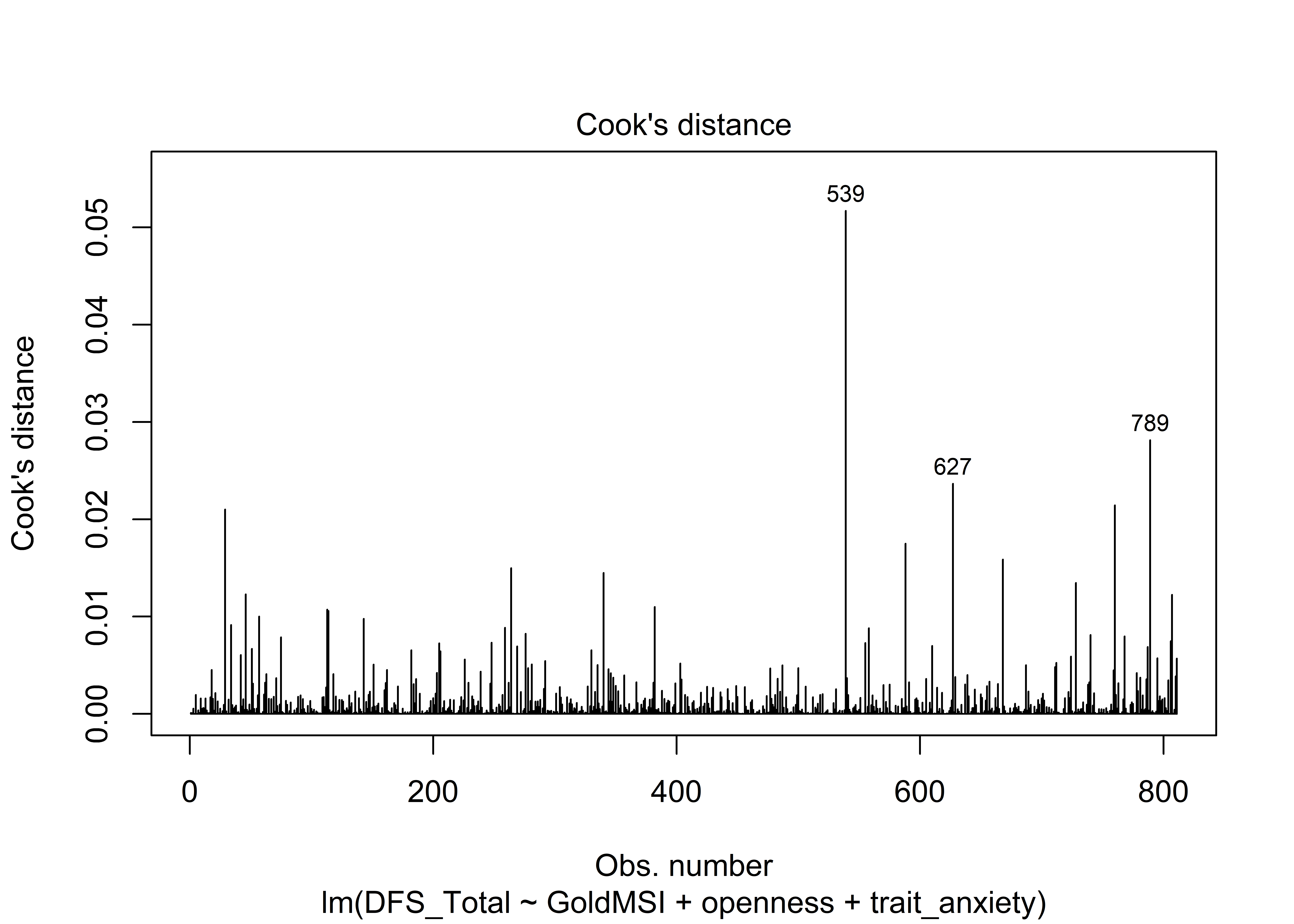
Base R also provides an easy way of visualising Cook’s distances in regression models using plot(). To do this, you just feed in the name of the regression model (much like how you check for homoscedasticity during regression diagnostics). Note that which = 4 must be specified.

plot(flow_block3, which = 4)

R will automatically label points that it thinks are influential data points in this plot. Based on this, data points 539, 627 and 789 might be worth a closer look.

How might you identify influential data points in general? There are many rules of thumb out there for Cook’s distances. Cook’s original guideline was to flag any point with a distance > 1, but this might be relatively rare (note that our maximum distance in this model is 0.05!). Other rules include \(\frac{2k}{4}\), where k is the number of predictors in the model, \(\frac{4}{n}\) where n = sample size, and \(2\sqrt{\frac{k}{n}}\). Truthfully, there is no singular metric that applies, so it’s up to you to choose one and apply it consistently.

10.4.2 Mahalanobis’ distance, \(D^2\)

Mahalanobis’ distance, \(D^2\), is a measure of multivariate outliers - ie. outliers across two or more predictors. The basic idea is that it is the literal distance between a ‘cloud’ of all of the predictors in your model. Outliers can be described as data points that are the furthest away from the centre of this ‘cloud’, quantified by having a high Mahalanobis distance.

Generating Mahalanobis’ distances in R is not difficult, and can be calculated using the mahalanobis_distance() function from the rstatix. This needs to be piped from the original dataset, and given the names of the predictors in the regression model.

In this case, as we are working with three predictors in this model - Gold-MSI scores, trait anxiety and openness - we give the names of these variables from our dataframe to this function.

flow_data <- flow_data %>%
  mahalanobis_distance(GoldMSI, trait_anxiety, openness)

flow_data

Note that this function will automatically flag whether a datapoint is an outlier. This is essentially done by calculating a critical Mahalanobis distance at p < .001. Any datapoint that sits above this critical Mahalanobis distance is flagged as an outlier (see expanded details below under “How do Mahalanobis distances work?”)

We can view which datapoints are flagged as outliers by simply filtering our dataset using filter():

flow_data %>%
  filter(is.outlier == TRUE)

Here, we can see that participants 378 and 528 are multivariate outliers, and thus we may want to consider doing something about them.

How do Mahalanobis distances work?

To calculate Mahalanobis distances by hand, you can use the mahalanobis() function from base R. To do this, you need to give the function a dataframe with just the predictors in it.

flow_temp <- flow_data %>%
  select(GoldMSI, trait_anxiety, openness)

head(flow_temp)

Then, feed it into the mahalanobis() function as below. Note the extra arguments; colMeans(flow_temp) specifies the means of the columns (i.e. the variables), and cov(flow_temp) generates the variance-covariance matrix between these variables.

mahal <- mahalanobis(flow_temp, colMeans(flow_temp), cov(flow_temp))

head(mahal)

## [1] 0.6491979 3.7060236 2.8816398 0.1675431 7.4849829 1.4083562

Mahalanobis distances follow a chi-square distribution. Thus, we can leverage the properties of the chi-square to calculate p-values for each Mahalanobis distance. For this test, degrees of freedom is equal to the number of predictors (i.e. df = 3 as we have three predictors).

p <- pchisq(mahal, df = 3, lower.tail = FALSE)

head(p)

## [1] 0.88508291 0.29500801 0.41023627 0.98265060 0.05794556 0.70357717

For Mahalanobis distances, the convention is to set the significance level at p < .001. Thus, at this point we can just go ahead and identify any data points that have a p-value below this cutoff.

Alternatively - and this is what rstatix does - you can calculate the Mahalanobis distance corresponding to p = .001, which will tell you the critical Mahalanobis distance value for a significant outlier.

qchisq(0.999, df = 3)

## [1] 16.26624

This means that any Mahalanobis distance above 16.27 will be significant.

10.4.3 What happens if there is an outlier?

Say that you’ve identified a bona fide outlier in your data. What do you do with it?

In these kinds of scenarios, the best-practice approach will most likely involve doing a sensitivity analysis. Sensitivity analyses are a general technique that broadly refer to testing your analyses under different conditions to see whether they hold under said conditions. The basic idea here is that you run two versions of your analyses:

First, a version with the outliers.
Next, a version without the outliers.

The aim is to see whether the effect(s) of interest change as a result of excluding the outliers, and by how much.

Let’s see an example of this using the same model as before. Here is the original flow_block3 model, just under a different name now:

flow_lm1 <- lm(DFS_Total ~ GoldMSI + trait_anxiety + openness, data = flow_data)
summary(flow_lm1)

## 
## Call:
## lm(formula = DFS_Total ~ GoldMSI + trait_anxiety + openness, 
##     data = flow_data)
## 
## Residuals:
##      Min       1Q   Median       3Q      Max 
## -15.0424  -2.2409  -0.0931   2.1484  12.3474 
## 
## Coefficients:
##               Estimate Std. Error t value Pr(>|t|)    
## (Intercept)   21.08246    1.33150  15.834   <2e-16 ***
## GoldMSI        2.66545    0.19623  13.583   <2e-16 ***
## trait_anxiety -0.10662    0.01154  -9.237   <2e-16 ***
## openness       0.29958    0.13700   2.187   0.0291 *  
## ---
## Signif. codes:  0 '***' 0.001 '**' 0.01 '*' 0.05 '.' 0.1 ' ' 1
## 
## Residual standard error: 3.345 on 807 degrees of freedom
## Multiple R-squared:  0.2971, Adjusted R-squared:  0.2945 
## F-statistic: 113.7 on 3 and 807 DF,  p-value: < 2.2e-16

Now, let’s remove the two outliers that we identified using Mahalanobis distances. These were participants 378 and 528. We will use filter() for simplicity.

The code below lets us remove specific rows. Let’s break down what this does:

The exclamation mark ! before id means “not” - i.e. do not do what comes next.
The %in% operator is a special operator in R that checks if a vector of values is present in another vector.
Here, id %in% c(378, 528) essentially means to see whether the id column has a 378 and 528 in it. By wrapping this in filter() we are essentially telling R to filer the rows where id equals 378 and 528.

However, since all of that is preceded with the exclamation mark, the code is actually telling R to filter all the rows that are not id = 378 or 528 - in essence, it filters these rows out. It’s a bit complex, but it’s good to know as it applies to many scenarios!

flow_no_outliers <- flow_data %>%
  filter(!id %in% c(378, 528))

Now that we have a dataframe without the two outliers, let’s now refit our model. The only argument we need to change is the name of the dataset:

flow_lm2 <- lm(DFS_Total ~ GoldMSI + trait_anxiety + openness, data = flow_no_outliers)
summary(flow_lm2)

## 
## Call:
## lm(formula = DFS_Total ~ GoldMSI + trait_anxiety + openness, 
##     data = flow_no_outliers)
## 
## Residuals:
##      Min       1Q   Median       3Q      Max 
## -15.0449  -2.2436  -0.1038   2.1526  12.3581 
## 
## Coefficients:
##               Estimate Std. Error t value Pr(>|t|)    
## (Intercept)   21.15098    1.34199  15.761   <2e-16 ***
## GoldMSI        2.66601    0.19680  13.547   <2e-16 ***
## trait_anxiety -0.10694    0.01158  -9.232   <2e-16 ***
## openness       0.29029    0.14011   2.072   0.0386 *  
## ---
## Signif. codes:  0 '***' 0.001 '**' 0.01 '*' 0.05 '.' 0.1 ' ' 1
## 
## Residual standard error: 3.348 on 805 degrees of freedom
## Multiple R-squared:  0.2965, Adjusted R-squared:  0.2939 
## F-statistic: 113.1 on 3 and 805 DF,  p-value: < 2.2e-16

We can see that even without the outliers, the pattern of results is very similar to the original model we had above. Therefore, in this kind of setting we don’t really gain anything by removing the outliers, and we might choose to keep the original model. Every participant lost is power lost, and the more information we have, the better! However, if your results do change substantially after excluding outliers then you will need to examine the differences carefully.

There are other methods that you could consider:

Using a non-parametric test, which are not affected by outliers see the section on non-parametric tests
Transforming the data to ‘un-outlier’ the outliers - this can be tricky to interpret

Regardless, it is a good idea to report both versions of the model - with and without outliers - for transparency, to show that you have actively considered these residuals.