8.4 Assumption tests
As usual, there are several assumptions that we need to test for regressions. Some people call these regression diagnostics - they mean the same as assumption testing.
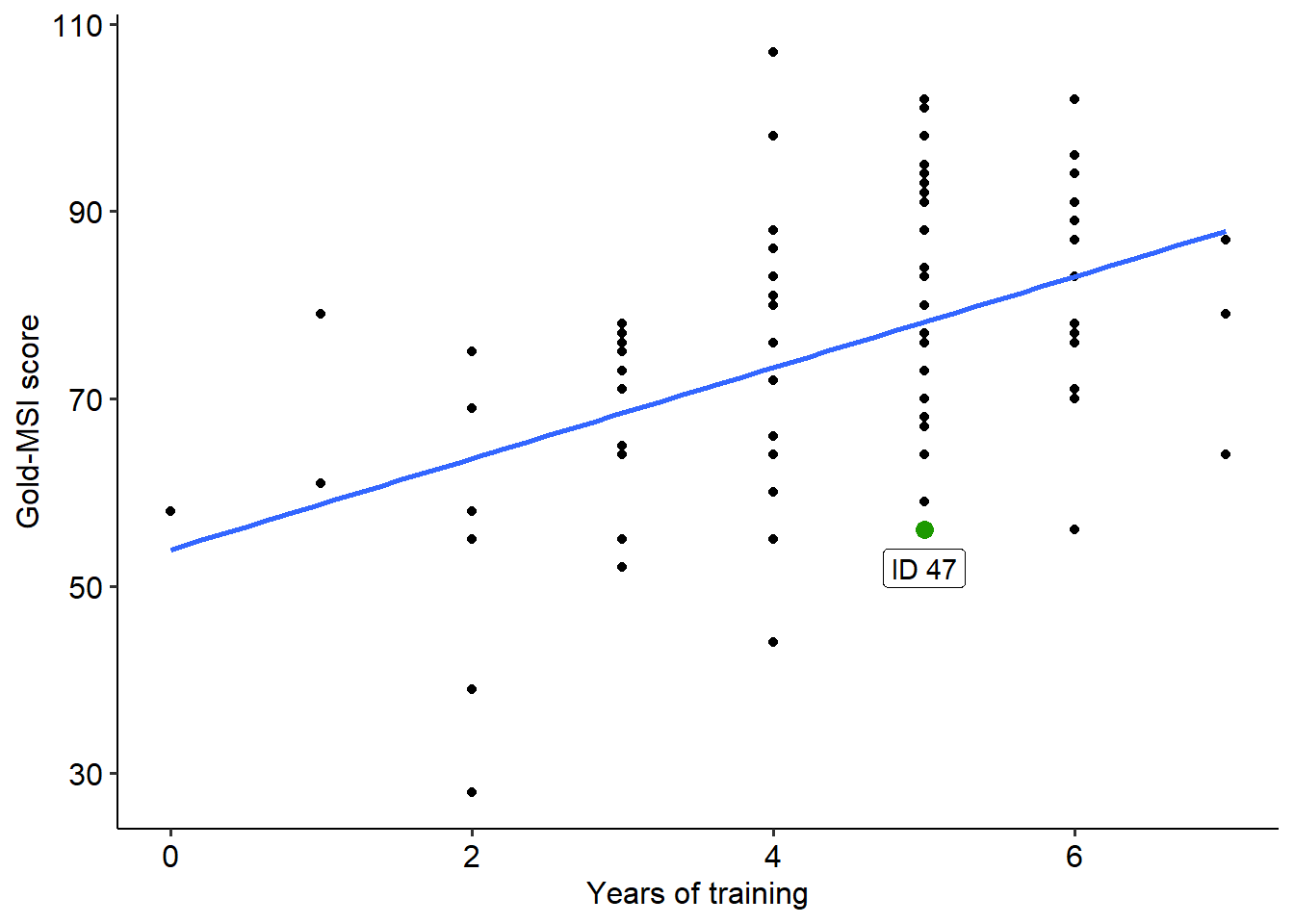
8.4.1 Linearity
Believe it or not, for a linear regression your data should be… linear. Wild, right?
Bitter sarcasm aside, linearity is an important assumption that needs to be met before conducting a linear regression. Not all data will follow a linear pattern; some data may instead sit on a curve. Compare the two examples below, where one is clearly non-linear:
If the data shows no clear linear relationship between your IV and DV, it is likely because the two are weakly correlated (and so a linear regression would not be useful anyway). If instead the data lies on a very obvious curve, you can either:
- Transform the data to make it linear (but you must be clear about what this represents)
- Attempt to fit a curve and see whether this has more explanatory power, but madness lies this way for the unprepared
8.4.2 Homoscedasticity
The homoscedasticity assumption is one that we’ve seen before - it is essentially a version of the equality of variance test. In a linear regression context, however, this assumption works a little bit differently; if this assumption is met, then the variance should be equal at all levels of our predictor (i.e. the x-axis).
The easiest way to test this is to create a fitted vs residuals graph. As the name implies, we take the fitted values for each level of the predictor in our data, and plot that against the residuals (fitted - actual). Here are some fitted vs residual plots for two sets of data. The data on the left has an even spread of variance as X increases, meaning that it is homoscedastic; the data on the right, on the other hand, spreads out like a cone. The data on the right therefore is likely heteroscedastic.
## Warning: Removed 7 rows containing missing values or values outside
## the scale range (`geom_point()`).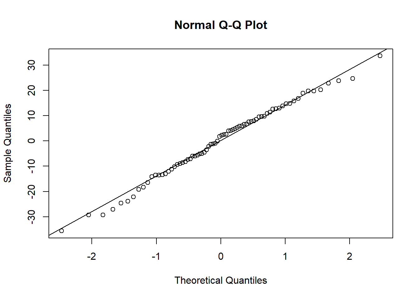
There are a couple of ways to overcome this, such as either transforming the raw variables or weighting them.
8.4.3 Independence
This one is the same - data points should be independent of each other. Like we have seen with other tests, this should ideally be a feature of good experimental design. In linear regression, a specific issue is autocorrelation - where the residuals between two values of X are not independent. If the residuals are not independent, your data likely exhibits signs of autocorrelation (i.e. it is correlated with itself). This can distort the relationship between your IV and DV, and indicates that your data are connected through time.
We can test this using a test called the Durbin-Watson test of autocorrelation. The Durbin-Watson test will estimate a coefficient/test statistic that quantifies the degree of autocorrelation (dependence) between observations in the data. The DW test statistic ranges from 0 to 4, with the following interpretations:
- A DW test statistic of ~2 indicates no autocorrelation.
- A DW test statistic of < 2 indicate positive autocorrelation - i.e. one data point will positively influence the next.
- A DW test statistic of > 2 indicates negative autocorrelation.
The general principle of the Durbin-Watson test, therefore, is to have a test statistic close to 2 and (ideally) a non-significant result. The value of the test statistic is generally more useful than the significance of the test alone. A common guideline for interpreting this value is that a DW test statistic below 1 or above 3 is problematic, which we will also use for this subject.
The DurbinWatsonTest() function from the DescTools package will let us test this quite easily.
##
##  Durbin-Watson test
##
## data:  mod_1
## DW = 2.0317, p-value = 0.5619
## alternative hypothesis: true autocorrelation is greater than 0
8.4.4 Normality
The normality assumption is the same here as it has been elsewhere - the residuals must be normally distributed. Here, it’s a little bit easier to visualise what these ‘residuals’ are because we can calculate and see them. That being said, the way we test for these are exactly the same - either use a Q-Q plot or a Shapiro-Wilks test.
8.4.5 Multicollinearity
The multicollinearity (sometimes just called collinearity) assumption only applies to multiple regressions, where you have more than one predictor in your test. multicollinearity occurs when two predictors are too similar to one another (i.e. they are highly correlated with each other. This becomes a problem at the individual predictor level, because what happens is that the effect of predictor A becomes muddled by predictor B - in other words, if two predictors are collinear, it becomes impossible to tell apart which one is contributing what to the regression.
There are three basic ways you can assess this.
- The simplest is to test a correlation between the two predictors. If they are very highly correlated (use r = .80 as a rule of thumb), this is likely to be a problem.
- The variance inflation factor (VIF) is a more formal measure of multicollinearity. It is a single number, and a higher value means greater collinearity. If a VIF is greater than 5 this suggests an issue.
- Tolerance is a related value to VIF - in fact, it is just 1 divided by the FID - and works in much the same way - except smaller values mean greater collinearity. As a rule of thumb, if tolerance is smaller than 0.20 this suggests an issue.
To calculate VIF, you can use the VIF() function from the DescTools package - more on the relevant page.