7.3 Multiple comparisons
On this page we talk about what happens after a significant ANOVA result, as well as some more detail about the multiple comparisons problem, and how it can be accounted for.
7.3.1 Post-hoc tests
The ANOVA table on the previous page allows us to calculate by hand whether there is a significant effect of our IV. However, it doesn’t tell us where that difference lies. Remember, we’re comparing at least three groups with each other - so we need some way of figuring out where the actual significant differences between means are.
Enter post-hoc comparisons (post-hoc = after the fact). These are essentially a series of t-tests where we compare each group with each other. So, if we have groups A, B and C, and we get a significant omnibus ANOVA that tells us there is a significant difference somewhere in those means, we would run post-hoc comparisons by running individual t-tests on A vs B, then B vs C, then A vs C.
However, we can’t just do this blindly, and there’s a good reason why…
7.3.2 The multiple comparisons problem
In Module 6, we talked a fair bit about Type I and II error rates - i.e., the rate of making a false positive and false negative judgement respectively. Here, we’ll focus on Type I error.
Recall that whenever we do a hypothesis test, we set a value for alpha, which forms our significance level. Alpha is essentially the probability of Type I errors we are willing to accept in a given test. In other words, when we use the conventional alpha = .05 as our criterion for significance, we are saying that we’re willing to accept a Type I error occurring 5% of the time - or 1 in 20.
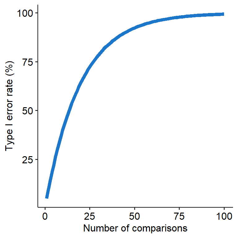
This becomes problematic when we have to conduct multiple tests at once, like what we have to do in an ANOVA. For example, let’s say a variable has 5 levels - A, B, C, D and E. If we ran an ANOVA on this data and found a significant omnibus effect, we would want to find out where that effect is. But that means that we’d have to compare A, B, C, D and E all against each other, in a round-robin tournament way (e.g. A vs B, then A vs C…). Where this becomes an issue is that each comparison will have its own 5% Type I error rate (assuming we use alpha = .05). So in this scenario, the Type I error rate will stack with each new comparison, meaning that our overall Type I error rate will climb higher and higher. This means that the chance of finding a false positive will increase (see graph below).
This overall rate of Type I errors is called the family-wise error rate (FWER). ‘Family’ in this context refers to a family of comparisons - like the comparison across A to E that we saw above.
7.3.3 Correction methods
One way of dealing with this is to correct the p-values to set the family-wise error rate back to 5%. We’ll go through three main types (two of which are already covered in the seminar).
Tukey’s HSD
Tukey’s Honest Significant Differences (Tukey HSD for short) is appropriate specifically for post-hoc tests after ANOVAs. It essentially works by first calculating the largest possible difference between each group’s means, then using that to calculate a critical mean difference. Any mean difference that is greater than this critical threshold is significant.
How does the Tukey test work?
Tukey’s HSD works very similarly in principle to a t-test, although the exact maths involved are slightly different. The test statistic for a Tukey test is called q which denotes the Studentized range distribution (a specific distribution). For a given comparison between two group means, the formula for q is:
\[ \Large q = \frac{|M_1 - M_2|}{SE} \]
Where \(M_1\) and \(M_2\) denote the means of groups 1 and 2, and SE denotes the standard error of the sum of the means. The q-statistic is then compared to a Studentized range distribution to estimate a p-value for that comparison. The shape of the Studentized range distribution is determined by alpha, k (the number of groups being compared) and df (in this case, the **error degrees of freedom***).Bonferroni
The Bonferroni correction is a method that can be used both within ANOVAs and in more general contexts. The Bonferroni correction works by multiplying each p-value in a set of comparisons by the number of comparisons (i.e. the number of p-values).
For example, if a set of comparisons gives the following p-values: 0.05, 0.25 and 0.10, we would apply a Bonferroni correction by multiplying each p-value by 3 (as there are 3 p-values) to get 0.15, 0.75 and 0.30 respectively.
(Note: in reality, Bonferroni works by dividing alpha by the number of comparisons, i.e. 0.05/3 - but for the purpose of significance testing, the maths works out to be the same).
Holm
The Holm correction is another correction method. In this method, each p-value is first ranked from smallest to largest. and then numbered in a descending fashion. Using the same p-values as above, we would get 0.05, 0.10 and 0.25. The p = .05 would be ranked as 3, the p = .10 would be 2 and p = .25 would be 1.
You then multiply the p-value by its rank, like the table below, to get your adjusted p-values:
| Original p-value | Sorted p-value | Rank | p-value x rank |
|---|---|---|---|
| 0.05 | 0.05 | 3 | 0.15 |
| 0.25 | 0.10 | 2 | 0.20 |
| 0.10 | 0.25 | 1 | 0.25 |
The Bonferroni procedure is very conservative, in that it may actually overcorrect (and subsequently reject too many); the Holm correction still corrects the overall FWER without also increasing the overall Type II rate as well.
7.3.4 Post-hocs in R
To just get adjusted p-values, we can use the function pairwise.t.test(). This needs three arguments:
xrefers to the column of data for the outcome, expressed asdata$x.grefers to the group/IV, again asdata$g.p.adjust.methodrefers to the adjustment method. Note this argument does not allow Tukey adjustments: only Bonferroni and Holm are allowed.
##
##  Pairwise comparisons using t tests with pooled SD
##
## data:  w9_slices$rating and w9_slices$group
##
##         caramel lemon
## lemon   0.6866  -
## vanilla 0.0541  0.0017
##
## P value adjustment method: bonferroni
A more powerful and flexible method is using the emmeans package. emmeans stands for estimated marginal means, which are model-derived estimates of each group’s mean. Simple effects tests are generally run on the estimate marginal means, and thus this package allows us a handy way to run these comparisons.
There are two steps to using emmeans:
- Define the estimated marginal means for the post-hocs.
This is simple to do. We call the emmeans() function, which will set up all comparisons for the post-hoc. This function needs two arguments at minimum:
- The
aovmodel name, and - The variable (i.e. the groups) from which you are comparing levels against. This is given as
~ group, where group denotes our IV.
Imagine an ANOVA model named model_aov, with variable A that defines the groups in our ANOVA. Our first step would be to set up the comparisons using emmeans() like below:
- Generate pairwise comparisons for the post-hoc.
Continuing on from the example above, we can use the pairs() function on our EM object, model_em, to run the post-hocs. infer = TRUE will generate confidence intervals for the difference in EM means. By default this will be set at 95% confidence, which is typically what we want.
If we want to adjust the p-values at this stage, we can give pairs() an additional argument adjust, with the name of the adjustment method as a string. pairs() will let you use Tukey, Bonferroni and Holm adjustments.
Optionally, to do this all in one go we could simply pipe from emmeans() to pairs() as follows: