13.5 Moderation: Example
To round this module off, here is a worked example of a moderation.
13.5.1 Example scenario
We will use the dataset from Powell et al. (2022) in the Week 10 seminar, which looks at harmonious and obsessive passion in the context of heavy metal music listeners. We’ll test a specific question for this example: Do positive experiences predict harmonious passion, and does satisfaction with life moderate this relationship?
13.5.2 Setting up in R
To set up a moderation using PROCESS, we turn to the process() function once again. This time, we want to set the following options:
wsets our moderator.model = 1indicates that we want a simple moderation.plot = 1gives us values for plotting the moderation.jn = 1calculates the Johnson-Neyman values for a significant moderation. These are also used for plotting.save = 2is used to save the output to a variable.
13.5.3 Output
Let’s now take a look at our output. The first output is our overall model fit, which is identical to what we get for any other multiple regression. Our model in this instance is significant, and explains 19.6% of the variance in harmonious passion.
The second output gives us our standard regression table. This tells us whether the moderation is significant, and we can interpret this as we would for any other regression we’ve seen. So, here we can see that positive experiences are a significant predictor of harmonious passion (B = 0.796, t = 6.290, p < .001), but satisfaction with life is not (p = .279). However, the interaction - or moderation - between the two is significant (B = 0.036, t = 2.576, p = .011).
##
## **************** PROCESS Procedure for R Version 5.0 ******************
##
##            Written by Andrew F. Hayes, Ph.D.  www.afhayes.com
##    Documentation available in Hayes (2022). www.guilford.com/p/hayes3
##
## ***********************************************************************
##
##   Model: 1
##       Y: HP_TOT
##       X: SPANE_pos
##       W: SWLS_TOT
##
## Sample size: 177
##
##
## ***********************************************************************
## Outcome Variable: HP_TOT
##
## Model Summary:
##           R      R-sq       MSE         F       df1       df2         p
##      0.4425    0.1958   32.2539   14.0427    3.0000  173.0000    0.0000
##
## Model:
##               coeff        se         t         p      LLCI      ULCI
## constant    26.4430    5.7267    4.6175    0.0000   15.1398   37.7462
## SPANE_pos    0.0960    0.2529    0.3796    0.7047   -0.4031    0.5951
## SWLS_TOT    -0.8896    0.3329   -2.6723    0.0083   -1.5466   -0.2325
## int_1        0.0358    0.0139    2.5757    0.0108    0.0084    0.0632
##
## Product terms key:
## int_1  :  SPANE_pos  x  SWLS_TOT
##
## Test(s) of highest order unconditional interaction(s):
##       R2-chng         F       df1       df2         p
## X*W    0.0308    6.6341    1.0000  173.0000    0.0108
## ----------
## Focal predictor: SPANE_pos (X)
##       Moderator: SWLS_TOT (W)
##
## Conditional effects of the focal predictor at values of the moderator(s):
##    SWLS_TOT    effect        se         t         p      LLCI      ULCI
##     12.0000    0.5256    0.1305    4.0288    0.0001    0.2681    0.7831
##     20.0000    0.8120    0.1290    6.2931    0.0000    0.5573    1.0666
##     28.0000    1.0984    0.2025    5.4242    0.0000    0.6987    1.4980
##
## Moderator value(s) defining Johnson-Neyman significance region(s):
##       Value   % below   % above
##      6.8962    4.5198   95.4802
##
## Conditional effect of focal predictor at values of the moderator:
##    SWLS_TOT    effect        se         t         p      LLCI      ULCI
##      5.0000    0.2750    0.1940    1.4176    0.1581   -0.1079    0.6579
##      6.5000    0.3287    0.1778    1.8485    0.0662   -0.0223    0.6796
##      6.8962    0.3429    0.1737    1.9738    0.0500    0.0000    0.6857
##      8.0000    0.3824    0.1627    2.3500    0.0199    0.0612    0.7035
##      9.5000    0.4361    0.1490    2.9264    0.0039    0.1420    0.7302
##     11.0000    0.4898    0.1371    3.5717    0.0005    0.2191    0.7604
##     12.5000    0.5435    0.1276    4.2606    0.0000    0.2917    0.7952
##     14.0000    0.5972    0.1209    4.9410    0.0000    0.3586    0.8357
##     15.5000    0.6509    0.1175    5.5379    0.0000    0.4189    0.8829
##     17.0000    0.7046    0.1179    5.9785    0.0000    0.4720    0.9372
##     18.5000    0.7583    0.1218    6.2259    0.0000    0.5179    0.9987
##     20.0000    0.8120    0.1290    6.2931    0.0000    0.5573    1.0666
##     21.5000    0.8657    0.1390    6.2263    0.0000    0.5912    1.1401
##     23.0000    0.9194    0.1513    6.0776    0.0000    0.6208    1.2179
##     24.5000    0.9731    0.1652    5.8887    0.0000    0.6469    1.2992
##     26.0000    1.0268    0.1805    5.6871    0.0000    0.6704    1.3831
##     27.5000    1.0805    0.1969    5.4883    0.0000    0.6919    1.4690
##     29.0000    1.1342    0.2140    5.3004    0.0000    0.7118    1.5565
##     30.5000    1.1879    0.2317    5.1267    0.0000    0.7305    1.6452
##     32.0000    1.2416    0.2499    4.9681    0.0000    0.7483    1.7348
##     33.5000    1.2953    0.2685    4.8241    0.0000    0.7653    1.8252
##     35.0000    1.3489    0.2874    4.6937    0.0000    0.7817    1.9162
##
## Data for visualizing the conditional effect of the focal predictor:
## SPANE_pos SWLS_TOT HP_TOT
## 19.0000 12.0000 25.7538
## 23.0000 12.0000 27.8561
## 27.0000 12.0000 29.9584
## 19.0000 20.0000 24.0785
## 23.0000 20.0000 27.3264
## 27.0000 20.0000 30.5742
## 19.0000 28.0000 22.4032
## 23.0000 28.0000 26.7966
## 27.0000 28.0000 31.1900##
## ******************** ANALYSIS NOTES AND ERRORS ************************
##
## Level of confidence for all confidence intervals in output: 95
##
## W values in conditional tables are the 16th, 50th, and 84th percentiles.This indicates that we should investigate further, first with our simple slope/interaction plot as below. Unfortunately, as you can tell, the plot argument in process() doesn’t actually generate any plots. Rather, it gives a series of values for the predictor, moderator and outcome to plot. The same applies for the output from the Johnson-Neyman technique - while the output does tell you where the moderation is/is not significant, it does not draw a plot. This is probably because PROCESS was designed for SPSS users first and foremost in mind, and the SAS and R versions were designed for parity for SPSS first and foremost (rather than designed to take advantage of their native capabilities).
There are ways to use these values for plotting, but truthfully - at least for this subject - they are far more effort than they are worth. Rather, there is a great package called interactions that will draw these plots for us.
To start, we use lm() to build a regular regression model with an interaction between our predictor and moderator:
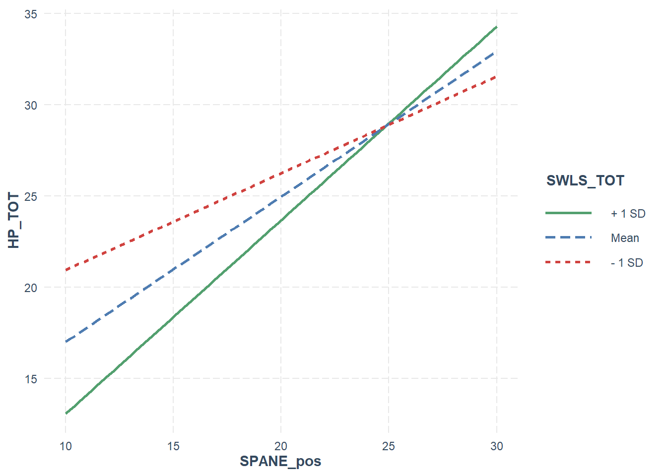
The interact_plot() function will then draw us a standard plot with simple slopes, based on the model above. For this function to work, at a minimum you must give it a) the name of the lm() model, b) the name of the predictor to pred and c) the name of the moderator to modx. The colors argument has also been specified to change the colours for the lines (by default they are different shades of blue).
Based on the below graph, we can see that in all instances, the relationship between positive experiences and harmonious passion is positive. However, for people who are high on satisfaction with like (Mean + 1SD), the relationship is stronger - indexed by a greater slope. This relationship is weaker for people who are low on satisfaction with life (Mean - 1SD).
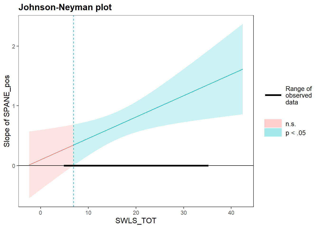
Lastly, we can examine the Johnson-Neyman plots to see where this relationship is non-significant. The same basic set of arguments - model, predictor, and moderator - can also be used as is for the johnson_neyman() function, which will draw a Johnson-Neyman plot. Helpfully, the function will also give a brief summary of the regions of significance/non-significance. Based on the plot and the text output, the moderation is non-significant when the moderator (satifaction with life) is below 6.9.
## JOHNSON-NEYMAN INTERVAL
##
## When SWLS_TOT is OUTSIDE the interval [-65.76, 6.90], the slope of
## SPANE_pos is p < .05.
##
## Note: The range of observed values of SWLS_TOT is [5.00, 35.00]