7.1 Anovas and the F-distribution
Just as we’ve done so for chi-squares and t-tests, let’s begin with an overview of the mathematical and conceptual underpinnings of the ANOVA.
7.1.1 The basic logic of ANOVAs
As we said in the introductory page, ANOVA stands for ANalysis Of VAriance. This essentially sums up how an ANOVA works in principle. ANOVAs can be used when analysing a categorical IV with two or more groups (typically 3+) and a continuous DV. As the setup suggests, ANOVAs are a good way of comparing different groups on a singular outcome.
The most basic hypotheses for an ANOVA center around whether or not the means between groups are significantly different, i.e.:
- \(H_0\): The means between groups are not significantly different. (i.e. \(\mu_1 = \mu_2 = ... \mu_k\))
- \(H_1\): The means between groups are significantly different. (i.e.\(\mu_1 \neq \mu_2 \neq ... \mu_k\))
How do we test for this? The basic logic of the ANOVA is this: Whenever we have data that we categorise into different groups, we end up with two key sources of variability, or variance: variance that exists between groups, and variance that exists within groups:
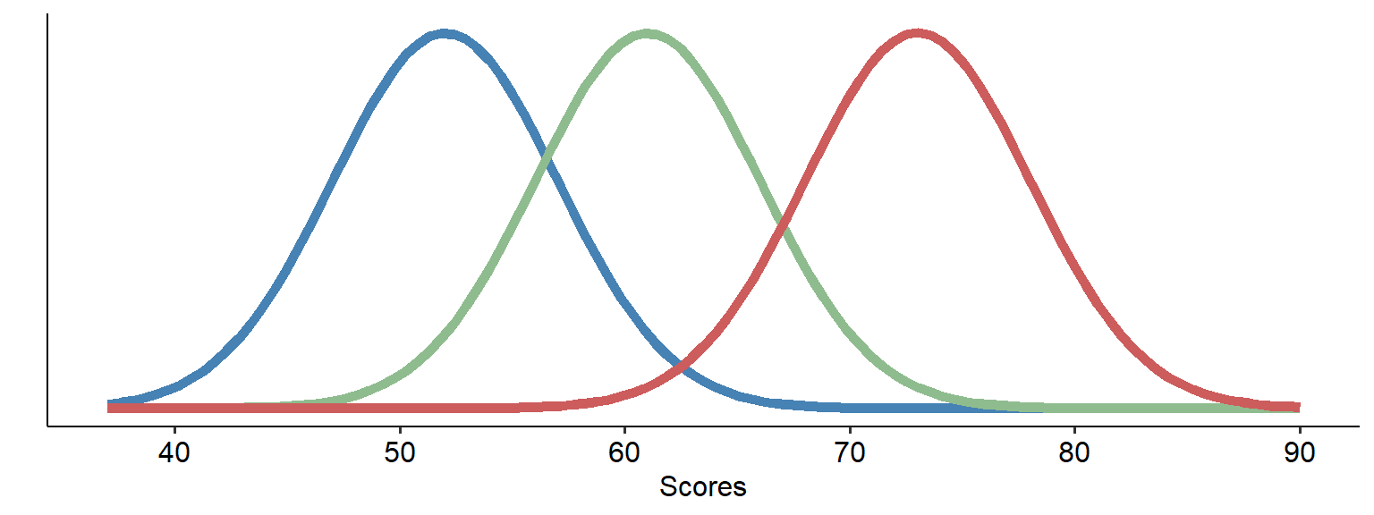
Pretend that the three curves above represent data covering three different groups, and that we’ve hypothesised that there are three different means. Collectively, this data has a certain amount of variance.
The first fundamental to recognise is that this total variance can be broken down into variance between groups and variance within groups:
\[ Variance_{total} = Variance_{between} + Variance_{within} \]
The variability between the groups would simply be the variance between the blue curve and the orange curve - in other words, how far apart the two sets of data are (in a simplistic sense). The within-group variance, on the other hand, is how much variance there is within each curve. If there is a lot of within-group variance within each curve, that would mean that (thinking back to Module 5) each group’s curve would be spread widely.
If you’re following the logic of this so far, the consequences of high within-group variance might be obvious - the two curves would significantly overlap. In contrast, if the between-group variance is far higher than the within-group variance, the curves may not overlap much at all - suggesting that the means of the two groups really are different.
This forms the basis of the ANOVA’s F-test, which is a ratio of variance:
\[ F = \frac{Variance_{between}}{Variance_{within}} \]
We will see this more in practice on the next page, but the F-statistic, which we use as part of significance testing in ANOVAs, is calculated by simply dividing the between-group variance by the within-group variance.
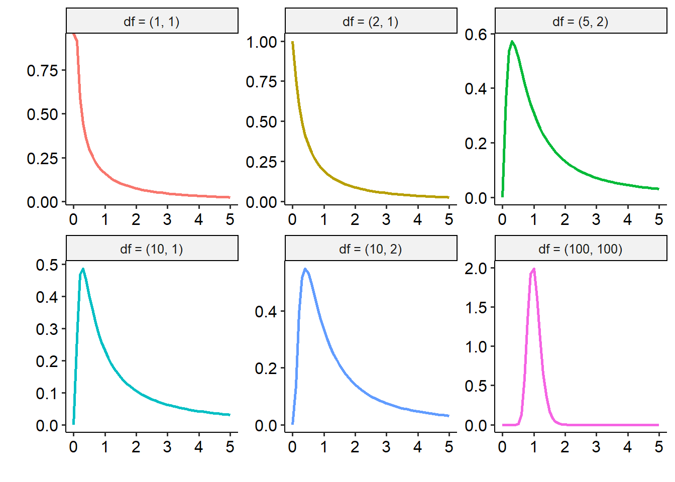
7.1.2 The F-distribution
Like the other tests we’ve encountered so far, ANOVAs have their own underlying distribution. In this instance, this is the F distribution, which describes how the F-statistic behaves. We won’t go far into the maths around this, but the key here is that the F distribution is characterised by two sets of degrees of freedom: one that relates to the between-groups variance/effect, and one that relates to the within-groups variance. One thing to note here is the terminology in the headers of each graph: the first number in the brackets refers to the between-groups variance, while the second number refers to the within-groups variance.
7.1.3 F-statistic tables
And, once again, we have a special F-table to determine critical F values, given two degrees of freedom values. However, given that we have two degrees of freedom the process is a little bit more complicated. Most F-stat tables actually provide multiple tables, corresponding to different alpha levels. For now, we will always use the table corresponding to alpha = 0.05, a snippet of which is below:
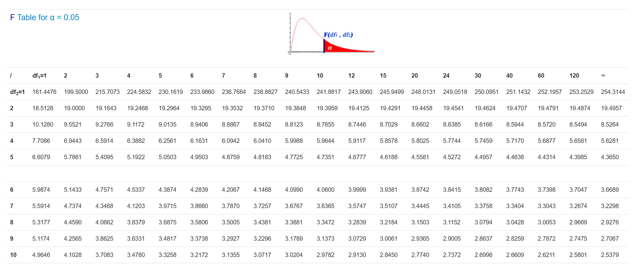
To read this table, you need to know both degrees of freedom (more on how to find that on the next page). The columns, marked df1, refer to the first df value (between-groups), while the rows correspond to the second df value (within-groups).
So, for example, if we have an F-test with degrees of freedom of (4, 10), we would first need to find the column that corresponds to 4 (our df1), and then the row that corresponds to df2 = 10. Reading the cell at the intersection would give us a critical F-statistic of 3.48; this is the value our F-statistic would need to be greater than to be significant at the p < .05 level.