7.2 The ANOVA table
Every time we do an ANOVA, there are actually a raft of calculations that have to occur in order to get our test statistic and p-value. Statistical software will display all of this in the form of an ANOVA table, which we cover below.
Don’t stress too much about the maths here - while the quiz does include one question about this, the question itself isn’t difficult (and you won’t be expected to do any of this by hand otherwise). The reason why we go through this, however, is to demonstrate the conceptual logic from the previous page.
7.2.1 The ANOVA table
On the previous page, we talked in depth about how the F statistic is calculated, and what shapes the overall distribution. But how do we actually calculate all of that stuff to begin with from raw data? Enter the ANOVA table, a beautiful (remember, beauty is subjective) way of calculating this information and laying it all out to see.
The basic ANOVA table looks like this, which you will see on any statistical package you use.
| Sums of squares (SS) | Degrees of freedom (df) | Mean square (MS) | F | p | |
|---|---|---|---|---|---|
| Group (our effect) | |||||
| Error/Residual | |||||
| Total |
A couple of terminology-related things here.
- ‘Group’ in this context is our independent variable (i.e. the effect of group)- this is our between-subject variance.
- ‘Error’ or ‘Residual’ is the within-group variance.
Let’s use the below data to calculate this by hand.
| Group 1 | Group 2 | Group 3 |
|---|---|---|
| 1 | 2 | 5 |
| 2 | 4 | 8 |
| 3 | 5 | 6 |
| 2 | 3 | 7 |
| Mean: 2 | Mean: 3.5 | Mean: 6 |
The grand mean (i.e. the mean across all 12 pieces of data) is 4. Keep this in mind.
Time to strap in - there are a lot of formulae involved!
7.2.2 Sums of squares
The sum of squares quantifies how far each observation is from the average - just like how it is calculated in the formula for standard deviations. For an ANOVA, we have two sets of SS to calculate - one for the between-groups term, and one for the within-groups/error.
Between
The formula for the between-groups sum of squares (\(SS_b\)) is:
\[ SS_b = \Sigma n(\bar x - \bar X)^2 \]
In words, this means:
- Take each group’s mean (\(\bar x\)), and subtract them from the grand mean (\(\bar X\))
- Square that difference
- Multiply it by n, the size of each group
- Add them all up.
Let’s do that for our fictional data. Our group means are Group 1 = 2, Group 2 = 3.5 and Group 3 = 6.5. \(SS_b = 4(2-4)^2 + 4(3.5-4)^2 + 4(6.5-4)^2\) \(SS_b = (4 \times 4) + (4 \times 0.25) + (4 \times 6.25)\) \(SS_b = 42\)
Within
For the within-group sum of squares, the formula is:
\[ SS_w = \Sigma (x - \bar x)^2 \]
This one is a bit more tedious. It means:
- Take each observation (\(x\)), and subtract them from their group mean (\(\bar x\))
- Square that difference
- Add them all up.
So for our data, it would look something like.. \[ SS_w = (1-2)^2 + (2-2)^2 + (3-2)^2 + (2-2)^2 + (2-3.5)^2 + (4-3.5)^2 + (5-3.5)^2 + (3-3.5)^2 + (5-6.5)^2 + (8-6.5)^2 + (6-6.5)^2 + (7-6.5)^2 \] \[SS_w = 12\].
7.2.3 Degrees of freedom
Because we have a term for between-groups and within-groups effects, we also have degrees of freedom for both (think back to the previous page). Thankfully, unlike the mess above the formulae here are relatively simple.
Between
The between-groups df is given as:
\[ df_b = k - 1 \]
Where k = the number of groups. So, in our data, \(df_b = 3 -1 = 2\) (as we have 3 groups).
Within
The within-groups df is given as:
\[ df_b = N - k \]
Where k = the number of groups, and N is the total sample size (in our case, 12). So \(df_w = 12 -3 = 9\) (as we have 3 groups and 12 data points in total).
7.2.4 Mean squares
The mean squares is another value for variance that essentially standardises the sum of squares by the degrees of freedom. The formula for MS between and within is the same:
\[ MS = \frac{SS}{df} \]
We’ve calculated SS and df for both our between and within-groups effects, so we can substitute these values in to calculate a mean square value for both:
\[MS_b = \frac{SS_b}{df_b}\] \[MS_w = \frac{SS_w}{df_w}\]
Putting in our values that we calculated earlier, we get:
\[MS_b = \frac{42}{2}\] \[MS_w = \frac{12}{9}\]
This gives us \(MS_b = 21\) and \(MS_w = 1.33\).
7.2.5 Calculating F
Remember on the previous page, how we talked about the F-statistic being a ratio between two variances (between divided by within)? That’s exactly what we’re going to do next, using our calculated mean-square values:
\[ F = \frac{MS_b}{MS_w} \]
This gives us:
\[ F = \frac{21}{1.33} = 15.75 \]
7.2.6 Putting it all together
Phew! Now we’ve calculated everything we need to for our ANOVA - in essence, we’ve done the majority of the ANOVA by hand. Let’s put all of our values into the table below:
| Sums of squares (SS) | Degrees of freedom (df) | Mean square (MS) | F | p | |
|---|---|---|---|---|---|
| Group (our effect) | 42 | 2 | 21 | 15.75 | |
| Error/Residual | 12 | 9 | 1.33 | ||
| Total | 54 |
Before we move on, it’s also worth noting that \(SS_b + SS_w = SS_{total}\) ; this goes back to the fundamental we discussed on the previous page, where an ANOVA breaks down total variance into between and within-groups variance.
7.2.7 Consulting the F-table
Now that we have our observed F-value, we can now consult an F-table and use our two degrees of freedom to find out what our critical F-value is (setting alpha = .05):
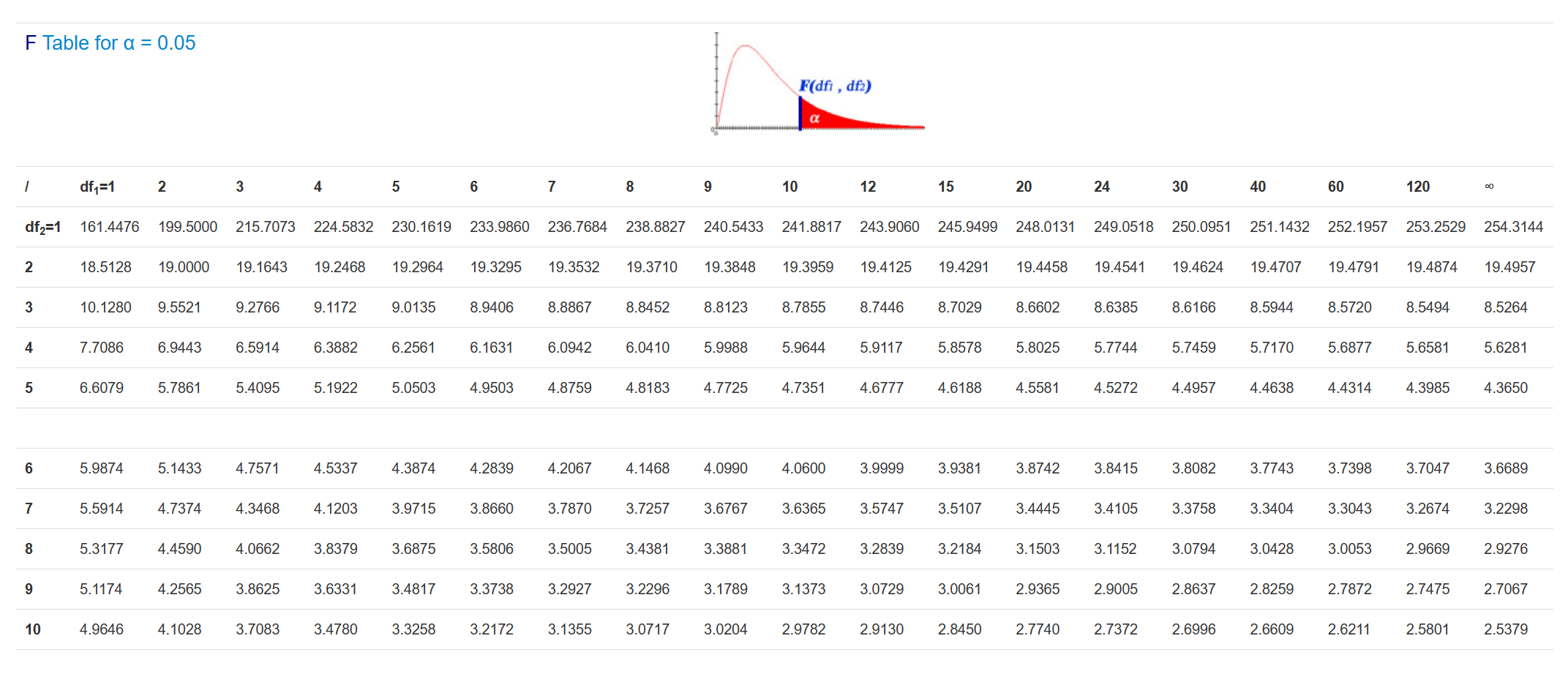
Reading the column for df1 = 2, and the row for df2 = 9, we get a critical F-statistic of 4.2565. Now we can say that because our observed test statistic (15.75) is greater than this critical value, our ANOVA is significant at the alpha = .05 level.
In reality, like many of the other tests, we would calculate a p-value by observing where our test statistic falls on the F-distribution, and the associated probability of getting that value or greater. Our software will do all of this stuff for us, but it helps to know exactly how an ANOVA works!
If you want to calculate the p-value manurally in R though, this is entirely possible using the pf() function:
## [1] 0.001149592