8.8 Multiple regressions in R
Phew - we’re almost there! Let’s round out this week’s module by doing a standard multiple regression in Jamovi.
8.8.1 Example data
Let’s look at a real set of data from Rakei et al. (2022). Their study looked at what predicts how prone people are to flow - the experience of being ‘in the moment’ and extremely focused while doing a task, such as performing. They measured a wide range of personality and emotion-related variables, but we’ll focus on just a subset here:
- Trait anxiety: broadly, refers to people’s tendency to feel anxious
- Openness to experience: a personality trait that describes how likely people are to seek new experiences
- DFS_Total: a measure of proneness to flow.
Let’s see if trait anxiety and openness predict flow proneness.
## Rows: 811 Columns: 6
## ── Column specification ───────────────────────────────────
## Delimiter: ","
## dbl (6): id, age, GoldMSI, DFS_Total, trait_anxiety, openness
##
## ℹ Use `spec()` to retrieve the full column specification for this data.
## ℹ Specify the column types or set `show_col_types = FALSE` to quiet this message.
To build a multiple regression model in R, we simply need to add (literally) more terms to lm():
8.8.2 Assumption checks
Our Durbin-Watson test suggests no issues with independence of observations.
##
##  Durbin-Watson test
##
## data:  w10_flow_lm
## DW = 1.9456, p-value = 0.2182
## alternative hypothesis: true autocorrelation is greater than 0
The Shapiro-Wilks test suggests that our normality assumption is violated - though if you look at the relevant Q-Q plot, it doesn’t appear to be very severe.
##
## Shapiro-Wilk normality test
##
## data: w10_flow_lm$residuals
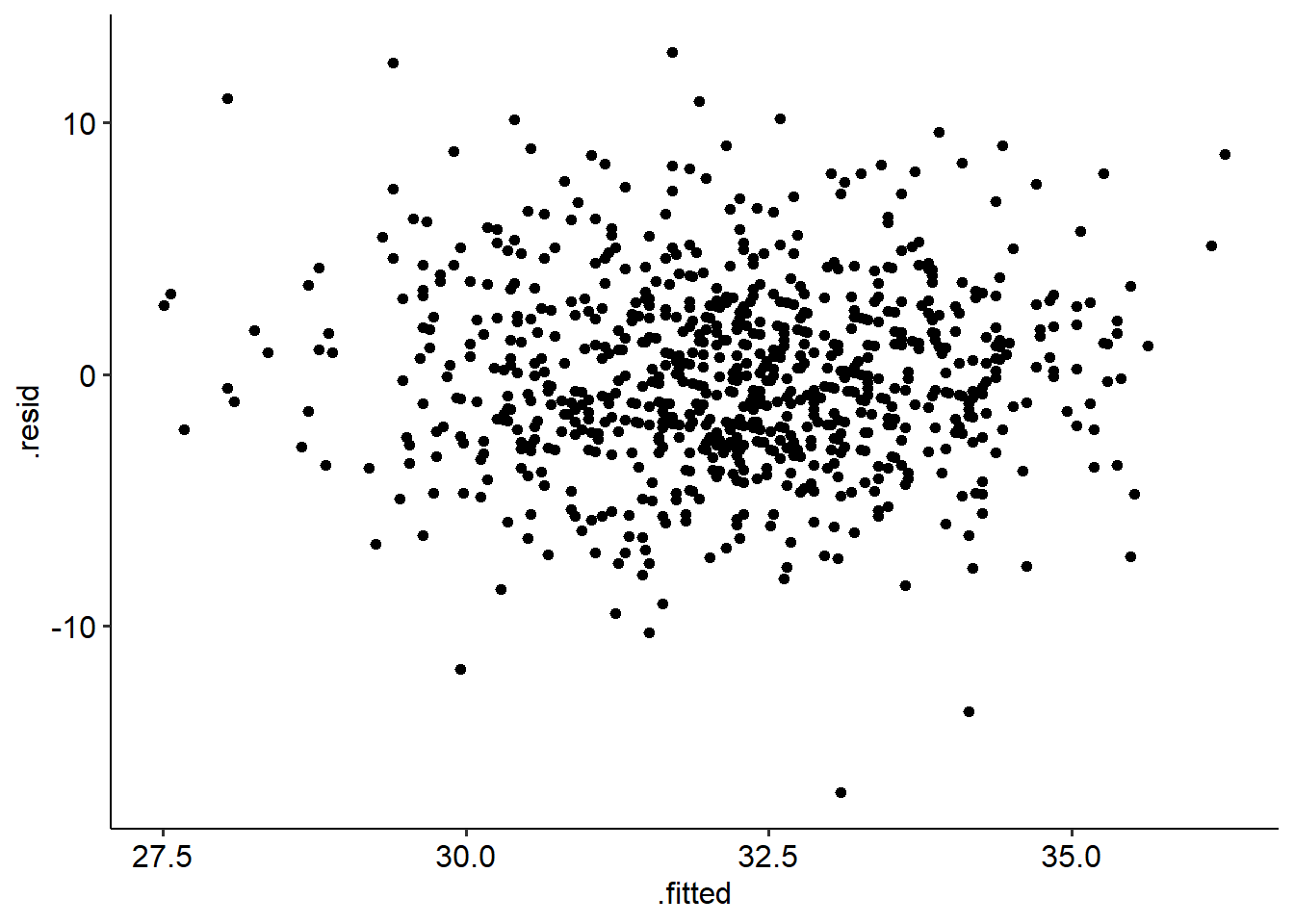
## W = 0.99311, p-value = 0.0008488The residuals-fitted plot for our data looks ok - no obvious conical shape, suggesting that the homoscedasticity assumption is intact.
Lastly, our multicollinearity statistics look good - no violations suggested here.
## trait_anxiety      openness
## 1.025955 1.025955## trait_anxiety openness
## 0.9747012 0.97470128.8.3 Output
Let’s start as always by taking a look at our output. Our regression explains 13.6 of the variance in flow proneness (\(R^2\) = .136), and our overall model is significant (F(2, 808) = 63.81, p < .001).
With that in mind, let’s turn to our individual predictors. Remember, now we have two predictors to consider - and we need to interpret them individually as well.
##
## Call:
## lm(formula = DFS_Total ~ trait_anxiety + openness, data = w10_flow)
##
## Residuals:
##     Min      1Q  Median      3Q     Max
## -16.596  -2.331  -0.151   2.308  12.794
##
## Coefficients:
##               Estimate Std. Error t value Pr(>|t|)
## (Intercept)   32.65078    1.13377  28.798  < 2e-16 ***
## trait_anxiety -0.11116    0.01278  -8.697  < 2e-16 ***
## openness       0.83372    0.14538   5.735 1.38e-08 ***
## ---
## Signif. codes:  0 '***' 0.001 '**' 0.01 '*' 0.05 '.' 0.1 ' ' 1
##
## Residual standard error: 3.705 on 808 degrees of freedom
## Multiple R-squared:  0.1364, Adjusted R-squared:  0.1343
## F-statistic: 63.81 on 2 and 808 DF, p-value: < 2.2e-16## 2.5 % 97.5 %
## (Intercept) 30.4252962 34.87625896
## trait_anxiety -0.1362446 -0.08606874
## openness 0.5483533 1.11907751We can see that both trait anxiety and openness are significant predictors of flow proneness, but interpreting the direction is also really important here. For that, we turn to our estimates:
- The estimate for trait anxiety is B = -.111 (95% CI [-.136, .086]), suggesting that higher trait anxiety predicts lower flow proneness (p < .001)
- On the other hand, the estimate for openness is B = .834 (95% CI [.548, 1.119]), suggesting that higher openness predicts higher flow proneness (p < .001).
Therefore, we can conclude that both are significant predictors and have opposite effects to each other. We can write this up as follows:
We ran a multiple regression with trait anxiety and openness as predictors, and flow proneness as an outcome. The overall regression model was significant (F(2, 808) = 63.81, p < .001), and explained 13.6% of the variance in flow proneness. Trait anxiety significantly predicted flow proneness (B = -.11, 95% CI [-.14, -.09], t = -8.70, p < .001); higher trait anxiety predicted lower flow proneness. Openness was also a significant predictor (B = .83, 95% CI [.55, 1.12], t = 5.74, p < .001); higher openness predicted higher flow proneness.
But there’s one more thing we can consider here…
8.8.4 Comparing predictive strength
When we do a multiple regression, we can actually identify which of our predictors is the strongest predictor of the outcome.
Our estimate column alone won’t tell us that, because these are unstandardised coefficients. They are unstandardised because they describe the relationship in terms of the original units of each measure. An increase of 1 unit on trait anxiety is not necessarily the same thing as a 1 unit increase in openness because they are on different scales, so we can’t compare them directly!
However, if we were to standardise these coefficients, we would then bring them all into the same scale (think back to z-scores!) - which would allow us to directly compare which predictor leads to a greater change in the outcome. These are simply regression coefficients that have been standardised, meaning that they are all on the same scale. Jamovi will calculate a standardised estimate (sometimes called standardised coefficient), which is presented in the rightmost column of the above table. Standardised estimates are denoted as beta (\(\beta\)), and thus are sometimes called standard betas.
Standard betas allow us to interpret our coefficients in terms of changes in standard deviations; namely, a 1 SD increase in predictor X leads to a \(\beta\) SD change in predictor Y.
In R, we need to use an extra function to calculate standard betas. We can call on the StdCoef() function from the DescTools package:
##                Estimate* Std. Error*  df
## (Intercept)    0.0000000   0.0000000 808
## trait_anxiety -0.2879944   0.0331142 808
## openness       0.1899044   0.0331142 808
## attr(,"class")
## [1] "coefTable" "matrix"
If you want confidence intervals around the standardised coefficients, the standardize_parameters() function from the effectsize package will do this for you:
Alternatively, we can simply standardise our predictors before running our regression (which is a lot easier in R than in other programs):
# Standardise predictors

w10_flow_std <- w10_flow %>%
  mutate(
    trait_anxiety = scale(trait_anxiety),
    openness = scale(openness),
    DFS_Total = scale(DFS_Total)
  )

w10_flow_lm_std <- lm(DFS_Total ~ trait_anxiety + openness, data = w10_flow_std)
summary(w10_flow_lm_std)
##
## Call:
## lm(formula = DFS_Total ~ trait_anxiety + openness, data = w10_flow_std)
##
## Residuals:
## Min 1Q Median 3Q Max
## -4.1675 -0.5855 -0.0379 0.5795 3.2128
##
## Coefficients:
## Estimate Std. Error t value Pr(>|t|)
## (Intercept) 9.281e-16 3.267e-02 0.000 1
## trait_anxiety -2.880e-01 3.311e-02 -8.697 < 2e-16 ***
## openness 1.899e-01 3.311e-02 5.735 1.38e-08 ***
## ---
## Signif. codes: 0 '***' 0.001 '**' 0.01 '*' 0.05 '.' 0.1 ' ' 1
##
## Residual standard error: 0.9304 on 808 degrees of freedom
## Multiple R-squared: 0.1364, Adjusted R-squared: 0.1343
## F-statistic: 63.81 on 2 and 808 DF, p-value: < 2.2e-16## 2.5 % 97.5 %
## (Intercept) -0.06413295 0.06413295
## trait_anxiety -0.35299439 -0.22299437
## openness 0.12490436 0.25490437This means that we can just compare the numbers of the standardised estimates (ignoring positive/negative signs) to see which one is the greatest predictor of the outcome. In the example above, trait anxiety has a standard coefficient of .288, whereas openness has a standard coefficient of .190. Trait anxiety is therefore a stronger predictor of flow proneness, because a 1 standard deviation increase in trait anxiety leads to a greater increase in flow proneness - namely, a change of .288 standard deviations.